class: center, middle, inverse, title-slide # <font class = "title-panel"> PPOL670 | Introduction to Data Science for Public Policy </font> <font size=6, face="bold"> Week 8 </font> <br> <br> <font size=100, face="bold"> Text as Data </font> ### <font class = "title-footer"> Prof. Eric Dunford ◆ Georgetown University ◆ McCourt School of Public Policy ◆ <a href="mailto:eric.dunford@georgetown.edu" class="email">eric.dunford@georgetown.edu</a></font> --- layout: true <div class="slide-footer"><span> PPOL670 | Introduction to Data Science for Public Policy           Week 8 <!-- Week of the Footer Here -->              Text-as-Data <!-- Title of the lecture here --> </span></div> --- class: outline # Outline for Today ![:space 10] - **String Manipulation** - **Text as "tidy" data** - **Sentiment Analysis** - **Topic Models** --- class: newsection # Strings --- ### String Manipulation in `R` .pull-left[  ] .pull-right[ ```r require(stringr) # or require(tidyverse) ``` ] -- ![:space 30] .center[ `str_<prefix>()` ```r str_c("a","b") ``` ``` ## [1] "ab" ``` ```r str_detect("There is a cat in the street",pattern = "cat") ``` ``` ## [1] TRUE ``` ] --- ![:space 20] ```r text = "There were 5 cats!" text ``` ``` ## [1] "There were 5 cats!" ``` -- ![:space 10] ```r str_view(text,"cats") ``` <div id="htmlwidget-a33436ac3cdeb0ac7508" style="width:960px;height:100%;" class="str_view html-widget"></div> <script type="application/json" data-for="htmlwidget-a33436ac3cdeb0ac7508">{"x":{"html":"<ul>\n <li>There were 5 <span class='match'>cats<\/span>!<\/li>\n<\/ul>"},"evals":[],"jsHooks":[]}</script> --- ### Regular Expressions (regex) .center[ |Regex | Description | |:----:|------------------------------| | `+` | match 1 or more of the previous character | | `*` | match 0 or more of the previous character | `?` |the preceding item is optional (i.e., match 0 or 1 of the previous character). | `[ ]` | match 1 of the set of things inside the bracket | `\\w` | match a "word" character (i.e., letters and numbers). | `\\d` | match digits | `\\s` | match a space character | `\\t` | match a "tab" character | `\\n` | match a "newline" character | `^` | the "beginning edge" of a string | `$` | the "ending edge" of a string | {n} | the preceding character is matched n times ] --- ![:space 30] ```r str_view(string = text, pattern = "\\d") ``` <div id="htmlwidget-56a43f716e2b9b07ef87" style="width:960px;height:100%;" class="str_view html-widget"></div> <script type="application/json" data-for="htmlwidget-56a43f716e2b9b07ef87">{"x":{"html":"<ul>\n <li>There were <span class='match'>5<\/span> cats!<\/li>\n<\/ul>"},"evals":[],"jsHooks":[]}</script> --- ![:space 30] ```r str_view_all(string = text, pattern = "\\s") ``` <div id="htmlwidget-b06161d820086d4c0654" style="width:960px;height:100%;" class="str_view html-widget"></div> <script type="application/json" data-for="htmlwidget-b06161d820086d4c0654">{"x":{"html":"<ul>\n <li>There<span class='match'> <\/span>were<span class='match'> <\/span>5<span class='match'> <\/span>cats!<\/li>\n<\/ul>"},"evals":[],"jsHooks":[]}</script> --- ![:space 30] ```r str_view_all(string = text, pattern = "\\d+\\s+\\w+") ``` <div id="htmlwidget-2a95a5790547650cb8f6" style="width:960px;height:100%;" class="str_view html-widget"></div> <script type="application/json" data-for="htmlwidget-2a95a5790547650cb8f6">{"x":{"html":"<ul>\n <li>There were <span class='match'>5 cats<\/span>!<\/li>\n<\/ul>"},"evals":[],"jsHooks":[]}</script> --- ### String Editing ![:space 5] ```r str_replace(string = text, pattern = "cats", replacement = "dogs") ``` ``` ## [1] "There were 5 dogs!" ``` -- ![:space 5] ```r str_remove(string = text, pattern = "[:punct:]") ``` ``` ## [1] "There were 5 cats" ``` -- ![:space 5] ```r str_extract(text,pattern = "\\d") ``` ``` ## [1] "5" ``` --- ### Locating text ```r texts <- c("The man drank 5 beers.", "Obama was president.", "I think we should walk 2 blocks.") ``` ![:space 5] ```r str_detect(texts,pattern = "\\d") ``` ``` ## [1] TRUE FALSE TRUE ``` ![:space 5] ```r str_which(texts,pattern = "\\d") ``` ``` ## [1] 1 3 ``` --- ### Insert data in a string ![:space 5] ```r x <- 10 str_c("The value is ",x,"%") ``` ``` ## [1] "The value is 10%" ``` -- ![:space 3] ```r x <- 10 str_glue("The value is {x}%") ``` ``` ## The value is 10% ``` -- ![:space 3] ```r x <- 10 str_glue("The value is {x + 5}%") ``` ``` ## The value is 15% ``` --- ### Capitalization ```r text2 <- "TeXt MininG iN r" ``` ```r str_to_lower(text2) ``` ``` ## [1] "text mining in r" ``` ```r str_to_upper(text2) ``` ``` ## [1] "TEXT MINING IN R" ``` ```r str_to_title(text2) ``` ``` ## [1] "Text Mining In R" ``` ```r str_to_sentence(text2) ``` ``` ## [1] "Text mining in r" ``` --- class: newsection # Tidy Text --- ![:space 20] .pull-left[  ] .pull-right[ <br><br><br> ```r require(tidytext) ``` ] --- ![:space 5] .pull-left[  ] .pull-right[ -  -  - : that require that the data be organized differently ] -- ![:space 65]  --- ![:space 5] .pull-left[  ] .pull-right[ **Tidy Text Data** - Each variable is a column - Each observation is a row - Each type of observational unit is a table tidy text format is a **table with one-token-per-row** ] ![:space 65]  --- ### Tokenization ![:space 5] ```r text ``` [1] "US opposition politicians and aid agencies have questioned a decision by President Donald Trump to cut off aid to three Central American states --- or so the story reports!" ```r text_data <- tibble(text = text) text_data ``` ``` ## # A tibble: 1 x 1 ## text ## <chr> ## 1 US opposition politicians and aid agencies have questioned a decision by Pres… ``` --- ### Tokenization (words) ```r text_data %>% unnest_tokens(word,text,token = "words") # Words are Default ``` ``` ## # A tibble: 28 x 1 ## word ## <chr> ## 1 us ## 2 opposition ## 3 politicians ## 4 and ## 5 aid ## 6 agencies ## 7 have ## 8 questioned ## 9 a ## 10 decision ## # … with 18 more rows ``` --- ### Tokenization (characters) ```r text_data %>% unnest_tokens(word,text,token = "characters") ``` ``` ## # A tibble: 140 x 1 ## word ## <chr> ## 1 u ## 2 s ## 3 o ## 4 p ## 5 p ## 6 o ## 7 s ## 8 i ## 9 t ## 10 i ## # … with 130 more rows ``` --- ### Tokenization (ngrams) ```r text_data %>% unnest_tokens(word,text,token = "ngrams",n=2) ``` ``` ## # A tibble: 27 x 1 ## word ## <chr> ## 1 us opposition ## 2 opposition politicians ## 3 politicians and ## 4 and aid ## 5 aid agencies ## 6 agencies have ## 7 have questioned ## 8 questioned a ## 9 a decision ## 10 decision by ## # … with 17 more rows ``` --- ### Tokenization (ngrams) ```r text_data %>% unnest_tokens(word,text,token = "ngrams",n=3) ``` ``` ## # A tibble: 26 x 1 ## word ## <chr> ## 1 us opposition politicians ## 2 opposition politicians and ## 3 politicians and aid ## 4 and aid agencies ## 5 aid agencies have ## 6 agencies have questioned ## 7 have questioned a ## 8 questioned a decision ## 9 a decision by ## 10 decision by president ## # … with 16 more rows ``` --- ### Tokenization (tweets) ```r tibble(text = "Hey @professor, this assignment doesn't make sense") %>% unnest_tokens(word,text,token = "tweets") %>% head(3) ``` ``` ## # A tibble: 3 x 1 ## word ## <chr> ## 1 hey ## 2 @professor ## 3 this ``` ```r tibble(text = "Hey @professor, this assignment doesn't make sense") %>% unnest_tokens(word,text,token = "words") %>% head(3) ``` ``` ## # A tibble: 3 x 1 ## word ## <chr> ## 1 hey ## 2 professor ## 3 this ``` --- ### From words to numbers (a.k.a. counting) Number of times a word appears in the text. ```r text_data %>% unnest_tokens(word,text) %>% count(word, sort = TRUE) ``` ``` ## # A tibble: 26 x 2 ## word n ## <chr> <int> ## 1 aid 2 ## 2 to 2 ## 3 a 1 ## 4 agencies 1 ## 5 american 1 ## 6 and 1 ## 7 by 1 ## 8 central 1 ## 9 cut 1 ## 10 decision 1 ## # … with 16 more rows ``` --- ### Stopwords Some words are common, carrying little to no _unique_ information, and need to be removed. `tidytext` comes with a database of common stop words, which we can leverage to remove these low information words. ```r set.seed(11) stop_words %>% sample_n(10) ``` ``` ## # A tibble: 10 x 2 ## word lexicon ## <chr> <chr> ## 1 anyone SMART ## 2 about snowball ## 3 large onix ## 4 everywhere SMART ## 5 worked onix ## 6 i snowball ## 7 say SMART ## 8 i'll SMART ## 9 been SMART ## 10 twice SMART ``` --- ### Drop Stopwords ```r text_data %>% unnest_tokens(word,text) %>% * anti_join(stop_words) %>% count(word,sort = T) ``` ``` ## # A tibble: 14 x 2 ## word n ## <chr> <int> ## 1 aid 2 ## 2 agencies 1 ## 3 american 1 ## 4 central 1 ## 5 cut 1 ## 6 decision 1 ## 7 donald 1 ## 8 opposition 1 ## 9 politicians 1 ## 10 president 1 ## 11 questioned 1 ## 12 reports 1 ## 13 story 1 ## 14 trump 1 ``` --- ### Stemming Often words are the same but appear different because of their tense. ```r txt = "cleaned cleaning cleaner beauty beautiful killing killed killer" tibble(text = txt) %>% unnest_tokens(word,text) %>% count(word) ``` ``` ## # A tibble: 8 x 2 ## word n ## <chr> <int> ## 1 beautiful 1 ## 2 beauty 1 ## 3 cleaned 1 ## 4 cleaner 1 ## 5 cleaning 1 ## 6 killed 1 ## 7 killer 1 ## 8 killing 1 ``` --- ### Stemming Stemming allows use to reduce a word down to it's fundamental root. ( _Note: Need to install `SnowballC` package_ ) ```r txt = "cleaned cleaning cleaner beauty beautiful killing killed killer" tibble(text = txt) %>% unnest_tokens(word,text) %>% * mutate(word = SnowballC::wordStem(word)) %>% count(word) ``` ``` ## # A tibble: 5 x 2 ## word n ## <chr> <int> ## 1 beauti 2 ## 2 clean 2 ## 3 cleaner 1 ## 4 kill 2 ## 5 killer 1 ``` --- ### Stemming ```r text_data %>% unnest_tokens(word,text) %>% anti_join(stop_words) %>% * mutate(word = SnowballC::wordStem(word)) %>% count(word,sort = T) ``` ``` ## # A tibble: 14 x 2 ## word n ## <chr> <int> ## 1 aid 2 ## 2 agenc 1 ## 3 american 1 ## 4 central 1 ## 5 cut 1 ## 6 decis 1 ## 7 donald 1 ## 8 opposit 1 ## 9 politician 1 ## 10 presid 1 ## 11 question 1 ## 12 report 1 ## 13 stori 1 ## 14 trump 1 ``` --- ### Example ```r require(rvest) urls <- c("https://www.bbc.com/news/election-us-2020-54437852", "https://www.bbc.com/news/world-us-canada-54441986", "https://www.bbc.com/news/election-us-2020-54423497") # Recall the BBC Scraper we build last class: news_data <- c() for(i in 1:length(urls)){ draw <- bbc_scraper(urls[i]) news_data <- bind_rows(news_data,draw) } ``` --- ### Example ```r news_data <- news_data %>% mutate(story_id = row_number()) # Create an id for the document glimpse(news_data) ``` ``` ## Rows: 3 ## Columns: 4 ## $ headline <chr> "Trump Covid: Biden warns there is 'a lot to be concerned ab… ## $ date <chr> "6 October 2020", "6 October 2020", "6 October 2020" ## $ story <chr> "Democratic presidential nominee Joe Biden has criticised US… ## $ story_id <int> 1, 2, 3 ``` --- ```r text_data <- news_data %>% group_by(story_id) %>% * unnest_tokens(word,story) %>% ungroup() text_data ``` ``` ## # A tibble: 2,894 x 4 ## headline date story_id word ## <chr> <chr> <int> <chr> ## 1 Trump Covid: Biden warns there is 'a lot to b… 6 October … 1 democrat… ## 2 Trump Covid: Biden warns there is 'a lot to b… 6 October … 1 presiden… ## 3 Trump Covid: Biden warns there is 'a lot to b… 6 October … 1 nominee ## 4 Trump Covid: Biden warns there is 'a lot to b… 6 October … 1 joe ## 5 Trump Covid: Biden warns there is 'a lot to b… 6 October … 1 biden ## 6 Trump Covid: Biden warns there is 'a lot to b… 6 October … 1 has ## 7 Trump Covid: Biden warns there is 'a lot to b… 6 October … 1 criticis… ## 8 Trump Covid: Biden warns there is 'a lot to b… 6 October … 1 us ## 9 Trump Covid: Biden warns there is 'a lot to b… 6 October … 1 president ## 10 Trump Covid: Biden warns there is 'a lot to b… 6 October … 1 donald ## # … with 2,884 more rows ``` --- ```r # Term Frequency text_data %>% group_by(story_id) %>% count(word,sort=T) ``` ``` ## # A tibble: 1,310 x 3 ## # Groups: story_id [3] ## story_id word n ## <int> <chr> <int> ## 1 1 the 74 ## 2 3 the 55 ## 3 1 to 52 ## 4 1 a 45 ## 5 1 he 31 ## 6 2 the 31 ## 7 1 and 29 ## 8 3 and 25 ## 9 1 of 22 ## 10 1 on 22 ## # … with 1,300 more rows ``` --- ```r ### Dropping stopwords text_data <- text_data %>% * anti_join(stop_words) text_data %>% group_by(story_id) %>% count(word,sort = T) ``` ``` ## # A tibble: 874 x 3 ## # Groups: story_id [3] ## story_id word n ## <int> <chr> <int> ## 1 1 trump 21 ## 2 1 president 17 ## 3 3 presidential 12 ## 4 3 debate 11 ## 5 1 house 10 ## 6 1 white 10 ## 7 1 coronavirus 9 ## 8 1 people 9 ## 9 2 positive 8 ## 10 2 president 8 ## # … with 864 more rows ``` --- Let's drop words that have digits in them... using regular expressions and the `stringr` package. ```r # Further Cleaning text_data %>% filter(str_detect(word,"\\d")) %>% select(story_id,word) ``` ``` ## # A tibble: 32 x 2 ## story_id word ## <int> <chr> ## 1 1 19 ## 2 1 3 ## 3 1 19 ## 4 1 19 ## 5 1 10 ## 6 1 19 ## 7 1 24 ## 8 1 7 ## 9 1 74 ## 10 1 12 ## # … with 22 more rows ``` --- Let's drop words that have digits in them... using regular expressions and the `stringr` package. ```r # Further Cleaning text_data <- text_data %>% filter(!str_detect(word,"\\d")) text_data %>% select(story_id,word) ``` ``` ## # A tibble: 1,262 x 2 ## story_id word ## <int> <chr> ## 1 1 democratic ## 2 1 presidential ## 3 1 nominee ## 4 1 joe ## 5 1 biden ## 6 1 criticised ## 7 1 president ## 8 1 donald ## 9 1 trump ## 10 1 downplaying ## # … with 1,252 more rows ``` --- ```r # Stemming text_data <- text_data %>% mutate(word = SnowballC::wordStem(word)) # Now count for real text_data_cnts <- text_data %>% group_by(story_id,headline) %>% count(word,sort=T) %>% ungroup() text_data_cnts ``` ``` ## # A tibble: 776 x 4 ## story_id headline word n ## <int> <chr> <chr> <int> ## 1 1 Trump Covid: Biden warns there is 'a lot to be conce… trump 21 ## 2 1 Trump Covid: Biden warns there is 'a lot to be conce… presid 17 ## 3 3 Kamala Harris v Mike Pence: Why this vice-president … debat 16 ## 4 3 Kamala Harris v Mike Pence: Why this vice-president … preside… 12 ## 5 1 Trump Covid: Biden warns there is 'a lot to be conce… hous 10 ## 6 1 Trump Covid: Biden warns there is 'a lot to be conce… white 10 ## 7 1 Trump Covid: Biden warns there is 'a lot to be conce… coronav… 9 ## 8 1 Trump Covid: Biden warns there is 'a lot to be conce… peopl 9 ## 9 2 Covid: US military leaders quarantine after official… chief 8 ## 10 2 Covid: US military leaders quarantine after official… posit 8 ## # … with 766 more rows ``` --- ### Inverse Document Frequency (tf-idf) Measures how important a word is given all words in the text. Mainly, we want to _up weight_ infrequently used words across the documents, and _down weight_ words that are used often by all the documents. <br> `$$idf(term) = ln(\frac{n_{documents}}{n_{documents~containing~term}})$$` `$$tf(term) = \frac{n_{word}}{n_{document}})$$` `$$tf\_idf(term) = tf(term)*idf(term)$$` ![:space 5] It's in the words particular to an author or document that the real information lies! --- ```r text_data_cnts2 <- text_data_cnts %>% bind_tf_idf(word, story_id, n) text_data_cnts2 %>% select(n,tf,idf,tf_idf) ``` ``` ## # A tibble: 776 x 4 ## n tf idf tf_idf ## <int> <dbl> <dbl> <dbl> ## 1 21 0.0339 0 0 ## 2 17 0.0275 0 0 ## 3 16 0.0455 0 0 ## 4 12 0.0341 0.405 0.0138 ## 5 10 0.0162 0.405 0.00655 ## 6 10 0.0162 0.405 0.00655 ## 7 9 0.0145 0.405 0.00590 ## 8 9 0.0145 0 0 ## 9 8 0.0275 0.405 0.0111 ## 10 8 0.0275 0 0 ## # … with 766 more rows ``` --- ### Visualize! ![:space 10] ```r text_data_cnts2 %>% group_by(story_id) %>% top_n(5, tf_idf) %>% ungroup() %>% mutate(word = reorder(word, tf_idf)) %>% ggplot(aes(word, tf_idf,fill=headline)) + geom_col(show.legend = F) + xlab(NULL) + coord_flip() + facet_wrap(~headline,ncol=1,scales="free") + theme(text=element_text(size=30)) ``` --- ### Visualize! <img src="lecture-week-08-text-as-data-ppol670_files/figure-html/unnamed-chunk-50-1.png" style="display: block; margin: auto;" /> --- class: newsection # Sentiment --- ![:space 25] 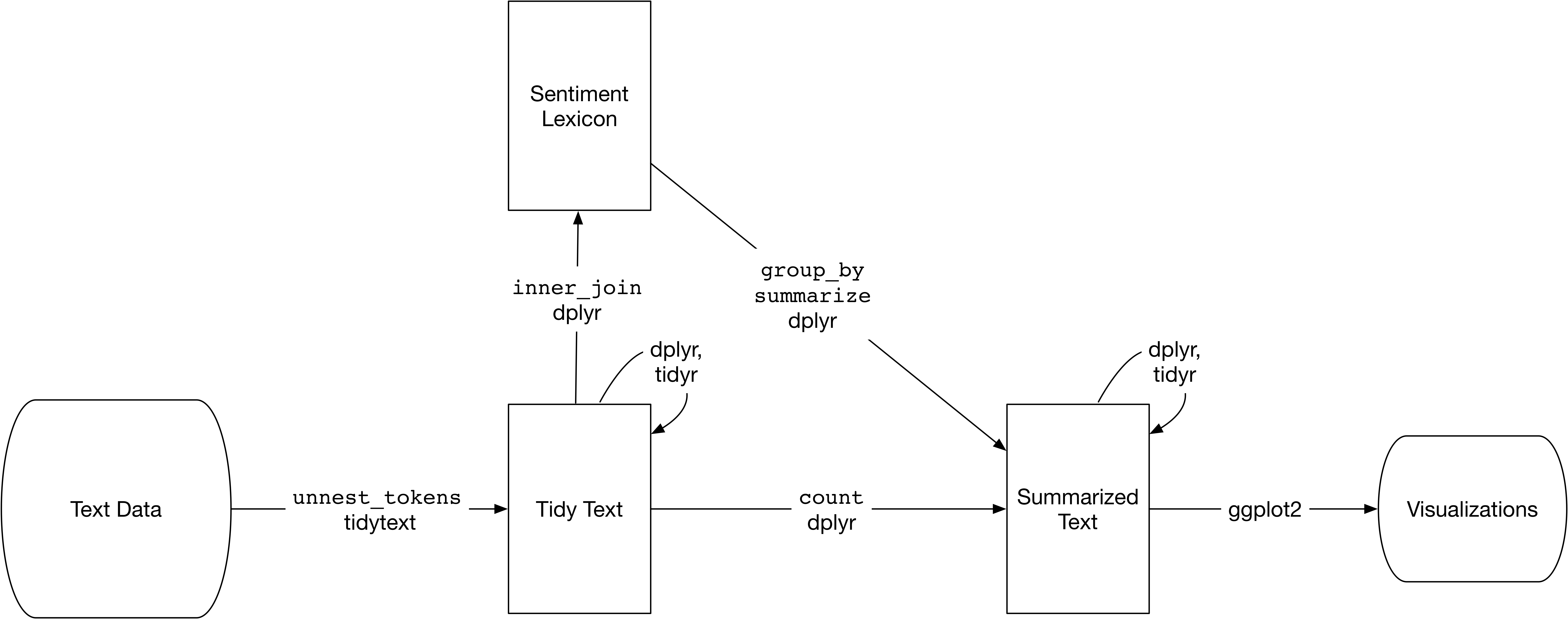 --- ### Sentiment Dictionaries ![:space 15] -- .center[ |Dictionary Name | Source |:----------------:|--------| | `nrc` | http://saifmohammad.com/WebPages/lexicons.html | `AFINN` | http://www2.imm.dtu.dk/pubdb/views/publication_details.php?id=6010 | `bing` | https://www.cs.uic.edu/~liub/FBS/sentiment-analysis.html | `loughran` | https://sraf.nd.edu/ ] --- ### Sentiment Dictionaries .pull-left[ ```r get_sentiments("afinn") ``` ``` ## # A tibble: 2,477 x 2 ## word value ## <chr> <dbl> ## 1 abandon -2 ## 2 abandoned -2 ## 3 abandons -2 ## 4 abducted -2 ## 5 abduction -2 ## 6 abductions -2 ## 7 abhor -3 ## 8 abhorred -3 ## 9 abhorrent -3 ## 10 abhors -3 ## # … with 2,467 more rows ``` ] .pull-right[ ```r get_sentiments("bing") ``` ``` ## # A tibble: 6,786 x 2 ## word sentiment ## <chr> <chr> ## 1 2-faces negative ## 2 abnormal negative ## 3 abolish negative ## 4 abominable negative ## 5 abominably negative ## 6 abominate negative ## 7 abomination negative ## 8 abort negative ## 9 aborted negative ## 10 aborts negative ## # … with 6,776 more rows ``` ] --- ### Sentiment to text ```r sent_dict <- get_sentiments("afinn") sent_text <- text_data %>% inner_join(sent_dict) %>% ungroup() sent_text ``` ``` ## # A tibble: 56 x 5 ## headline date story_id word value ## <chr> <chr> <int> <chr> <dbl> ## 1 Trump Covid: Biden warns there is 'a lot t… 6 October … 1 fear -2 ## 2 Trump Covid: Biden warns there is 'a lot t… 6 October … 1 glad 3 ## 3 Trump Covid: Biden warns there is 'a lot t… 6 October … 1 hope 2 ## 4 Trump Covid: Biden warns there is 'a lot t… 6 October … 1 matter 1 ## 5 Trump Covid: Biden warns there is 'a lot t… 6 October … 1 death -2 ## 6 Trump Covid: Biden warns there is 'a lot t… 6 October … 1 save 2 ## 7 Trump Covid: Biden warns there is 'a lot t… 6 October … 1 threat -2 ## 8 Trump Covid: Biden warns there is 'a lot t… 6 October … 1 prote… 1 ## 9 Trump Covid: Biden warns there is 'a lot t… 6 October … 1 danger -2 ## 10 Trump Covid: Biden warns there is 'a lot t… 6 October … 1 prote… 1 ## # … with 46 more rows ``` --- ```r sent_text %>% distinct(word,value) %>% * mutate(word = fct_reorder(word,value)) %>% ggplot(aes(word, value)) + geom_col(show.legend = FALSE,aes(fill=value)) + scale_fill_viridis_c() + coord_flip() + theme(text=element_text(size=20)) ``` <img src="lecture-week-08-text-as-data-ppol670_files/figure-html/unnamed-chunk-55-1.png" style="display: block; margin: auto;" /> --- ```r text_data %>% ungroup %>% inner_join(get_sentiments("bing"),by = "word") %>% distinct(word,sentiment) %>% mutate(word = fct_reorder(word,sentiment=="positive")) %>% ggplot(aes(word, sentiment,label=word,color=sentiment)) + geom_text(size=3,show.legend = FALSE) + coord_flip() + scale_color_manual(values=c("darkred","steelblue")) + theme_minimal() + theme(text=element_text(size=20),axis.text.y = element_blank()) ``` <img src="lecture-week-08-text-as-data-ppol670_files/figure-html/unnamed-chunk-56-1.png" style="display: block; margin: auto;" /> --- ### Example: Inaugural Speeches ```r inaug_dat <- read_csv("Data/inaug_speeches.csv") inaug_dat ``` ``` ## # A tibble: 58 x 5 ## X1 Name `Inaugural Address` Date text ## <dbl> <chr> <chr> <chr> <chr> ## 1 4 George W… First Inaugural Ad… Thursday, … "Fellow-Citizens of the Sena… ## 2 5 George W… Second Inaugural A… Monday, Ma… "Fellow Citizens: \xa0\xa0I… ## 3 6 John Ada… Inaugural Address Saturday, … "\xa0\xa0WHEN it was first p… ## 4 7 Thomas J… First Inaugural Ad… Wednesday,… "Friends and Fellow-Citizens… ## 5 8 Thomas J… Second Inaugural A… Monday, Ma… "\xa0\xa0PROCEEDING, fellow-… ## 6 9 James Ma… First Inaugural Ad… Saturday, … "\xa0\xa0UNWILLING to depart… ## 7 10 James Ma… Second Inaugural A… Thursday, … "\xa0\xa0ABOUT to add the so… ## 8 11 James Mo… First Inaugural Ad… Tuesday, M… "\xa0\xa0I SHOULD be destitu… ## 9 12 James Mo… Second Inaugural A… Monday, Ma… "Fellow-Citizens: \xa0\xa0I… ## 10 13 John Qui… Inaugural Address Friday, Ma… "\xa0\xa0IN compliance with … ## # … with 48 more rows ``` --- ### Example: Inaugural Speeches ```r obama <- inaug_dat %>% filter(Name == "Barack Obama") %>% select(address = `Inaugural Address`,text) obama ``` ``` ## # A tibble: 2 x 2 ## address text ## <chr> <chr> ## 1 First Inaugural Add… "My fellow citizens: \xa0\xa0I stand here today humbl… ## 2 Second Inaugural Ad… "Vice President Biden, Mr. Chief Justice, Members of the… ``` --- ### Example: Inaugural Speeches ```r obama_txt <- obama %>% unnest_tokens(word,text) %>% anti_join(stop_words) %>% inner_join(get_sentiments("afinn")) %>% group_by(address) %>% mutate(index = row_number()) %>% ungroup() obama_txt ``` ``` ## # A tibble: 300 x 4 ## address word value index ## <chr> <chr> <dbl> <int> ## 1 First Inaugural Address grateful 3 1 ## 2 First Inaugural Address trust 1 2 ## 3 First Inaugural Address peace 2 3 ## 4 First Inaugural Address vision 1 4 ## 5 First Inaugural Address faithful 3 5 ## 6 First Inaugural Address true 2 6 ## 7 First Inaugural Address crisis -3 7 ## 8 First Inaugural Address war -2 8 ## 9 First Inaugural Address reaching 1 9 ## 10 First Inaugural Address violence -3 10 ## # … with 290 more rows ``` --- ### Example: Inaugural Speeches ```r obama_txt %>% ggplot(aes(index,value,fill=address)) + geom_col(show.legend = FALSE) + facet_wrap(~address,ncol = 1, scales = "free_y") + theme_minimal() +theme(text = element_text(size=20)) ``` <img src="lecture-week-08-text-as-data-ppol670_files/figure-html/unnamed-chunk-60-1.png" style="display: block; margin: auto;" /> --- ### Example: Inaugural Speeches ![:space 15] ```r obama_txt %>% group_by(address) %>% summarize(proportion_words_positive = sum(value>0)/n()) ``` ``` ## # A tibble: 2 x 2 ## address proportion_words_positive ## <chr> <dbl> ## 1 First Inaugural Address 0.589 ## 2 Second Inaugural Address 0.657 ``` --- ### Example: Inaugural Speeches ![:space 10] ```r obama_txt %>% group_by(word,address) %>% summarize(n = n(),score=max(value)) %>% filter(n>1) %>% ggplot(aes(label=word,size=n,color=score)) + * ggwordcloud::geom_text_wordcloud_area() + scale_color_gradient(low="darkred",high="steelblue") + scale_size_area(max_size = 15) + facet_wrap(~address,scales="free") + theme(text = element_text(size=20)) ``` --- ### Example: Inaugural Speeches <img src="lecture-week-08-text-as-data-ppol670_files/figure-html/unnamed-chunk-63-1.png" style="display: block; margin: auto;" /> --- class: newsection # Topic Models --- ![:space 10] 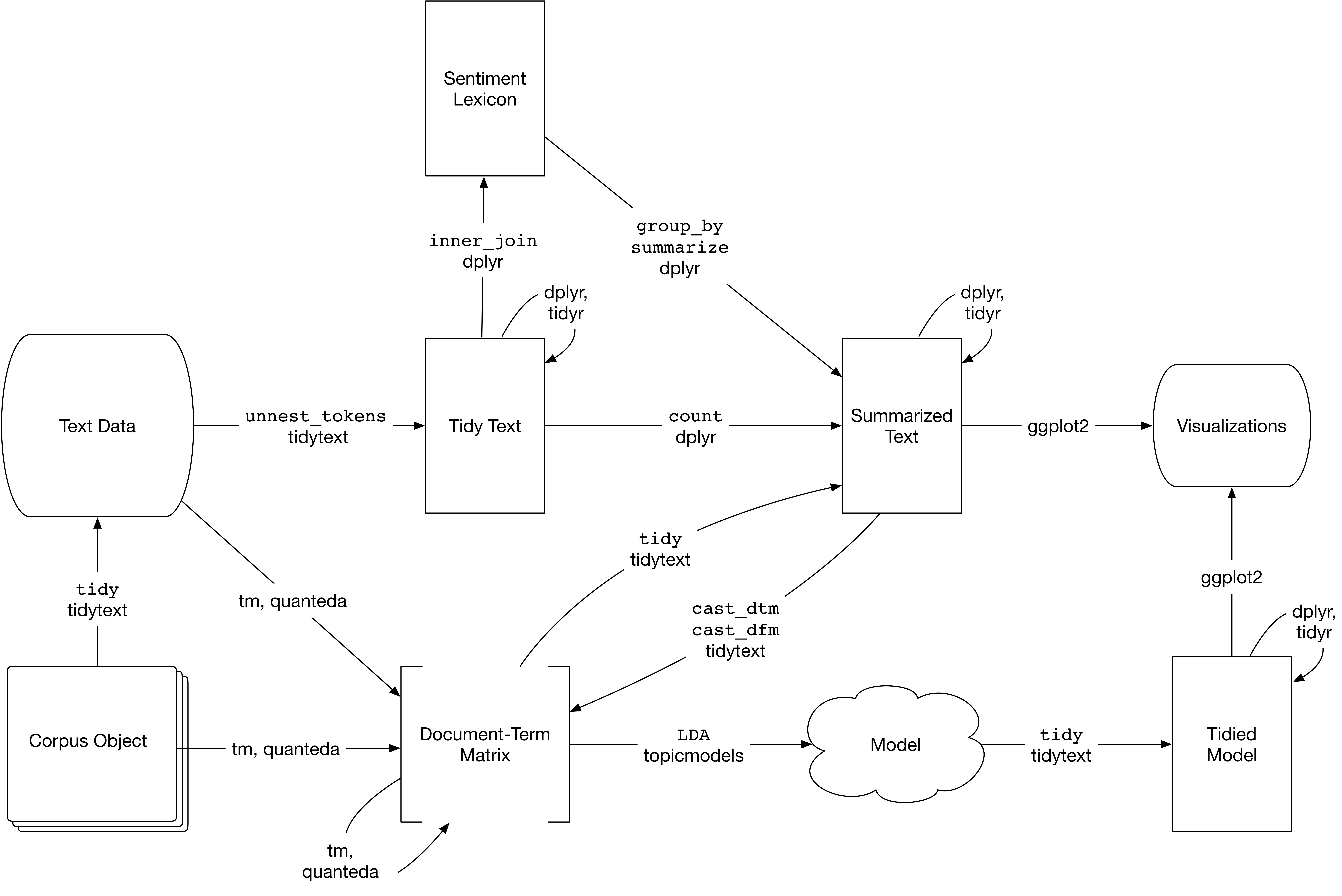 --- ### Latent Dirichlet Allocation (LDA) - **Every document is a mixture of topics** - We could imagine a two-topic model of American news, with one topic for “politics” and one for “entertainment.” - We could say “Document 1 is 90% about "politics" and 10% about "entertainment", while Document 2 is 30% about "politics" and 70% about "entertainment." - **Every topic is a mixture of words** - The most common words in the "politics" topic might be “President”, “Congress”, and “government”, while the entertainment topic may be made up of words such as “movies”, “television”, and “actor”. - Words can be shared between topics; a word like “budget” might appear in both equally. --- ### Latent Dirichlet Allocation (LDA) ![:space 10] 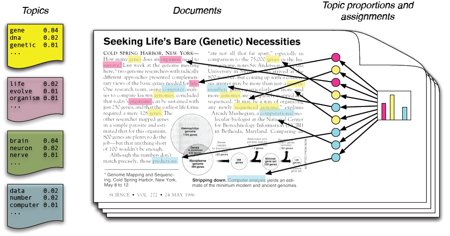 --- ```r library(topicmodels) data("AssociatedPress") AssociatedPress ``` ``` ## <<DocumentTermMatrix (documents: 2246, terms: 10473)>> ## Non-/sparse entries: 302031/23220327 ## Sparsity : 99% ## Maximal term length: 18 ## Weighting : term frequency (tf) ``` -- Can convert easily from a document term matrix (see reading) back to a tidy text format with `tidy()` ```r AssociatedPress %>% tidy() ``` ``` ## # A tibble: 302,031 x 3 ## document term count ## <int> <chr> <dbl> ## 1 1 adding 1 ## 2 1 adult 2 ## 3 1 ago 1 ## 4 1 alcohol 1 ## 5 1 allegedly 1 ## 6 1 allen 1 ## 7 1 apparently 2 ## 8 1 appeared 1 ## 9 1 arrested 1 ## 10 1 assault 1 ## # … with 302,021 more rows ``` --- ### LDA ```r ap_lda <- LDA(AssociatedPress, k = 2, control = list(seed = 1234)) ap_lda ``` ``` ## A LDA_VEM topic model with 2 topics. ``` ![:space 15] - Like the other clustering methods that we encountered, `k` is arbitrary. Here we shot for `\(k = 2\)` - Running an LDA is _easy_ (though they are computationally expensive) - The challenge lies in **interpreting** the topic output. --- - Extract information regarding topic assignment using the `tidy()` function from the `tidytext` package - Parameters of interest - "beta" → Term to Topic - "gamma" → Document to Topic ```r ap_topics <- tidy(ap_lda, matrix = "beta") ap_topics ``` ``` ## # A tibble: 20,946 x 3 ## topic term beta ## <int> <chr> <dbl> ## 1 1 aaron 1.69e-12 ## 2 2 aaron 3.90e- 5 ## 3 1 abandon 2.65e- 5 ## 4 2 abandon 3.99e- 5 ## 5 1 abandoned 1.39e- 4 ## 6 2 abandoned 5.88e- 5 ## 7 1 abandoning 2.45e-33 ## 8 2 abandoning 2.34e- 5 ## 9 1 abbott 2.13e- 6 ## 10 2 abbott 2.97e- 5 ## # … with 20,936 more rows ``` --- ```r ap_top_terms <- ap_topics %>% group_by(topic) %>% # Group by the topics # Grab the top 10 words most # associated with the topic top_n(10, beta) %>% ungroup() %>% # Ungroup arrange(topic, -beta) # Arrange ap_top_terms ``` ``` ## # A tibble: 20 x 3 ## topic term beta ## <int> <chr> <dbl> ## 1 1 percent 0.00981 ## 2 1 million 0.00684 ## 3 1 new 0.00594 ## 4 1 year 0.00575 ## 5 1 billion 0.00427 ## 6 1 last 0.00368 ## 7 1 two 0.00360 ## 8 1 company 0.00348 ## 9 1 people 0.00345 ## 10 1 market 0.00333 ## 11 2 i 0.00705 ## 12 2 president 0.00489 ## 13 2 government 0.00452 ## 14 2 people 0.00407 ## 15 2 soviet 0.00372 ## 16 2 new 0.00370 ## 17 2 bush 0.00370 ## 18 2 two 0.00361 ## 19 2 years 0.00339 ## 20 2 states 0.00320 ``` --- ### Deciphering the Topics ```r ap_top_terms %>% mutate(term = reorder(term, beta)) %>% ggplot(aes(term, beta, fill = factor(topic))) + geom_col(show.legend = FALSE) + facet_wrap(~ topic, scales = "free") + coord_flip() + theme(text=element_text(size=16)) ``` <img src="lecture-week-08-text-as-data-ppol670_files/figure-html/unnamed-chunk-69-1.png" style="display: block; margin: auto;" /> --- ### Documents to Topics ```r ap_documents <- tidy(ap_lda, matrix = "gamma") %>% arrange(document,gamma) ap_documents ``` ``` ## # A tibble: 4,492 x 3 ## document topic gamma ## <int> <int> <dbl> ## 1 1 1 0.248 ## 2 1 2 0.752 ## 3 2 1 0.362 ## 4 2 2 0.638 ## 5 3 2 0.473 ## 6 3 1 0.527 ## 7 4 1 0.357 ## 8 4 2 0.643 ## 9 5 1 0.181 ## 10 5 2 0.819 ## # … with 4,482 more rows ``` --- ### Documents to Topics Document #6 is highly associated with the "politics" topic ```r ap_documents %>% filter(document==6) ``` ``` ## # A tibble: 2 x 3 ## document topic gamma ## <int> <int> <dbl> ## 1 6 1 0.000588 ## 2 6 2 0.999 ``` ```r tidy(AssociatedPress) %>% filter(document == 6) %>% arrange(desc(count)) ``` ``` ## # A tibble: 287 x 3 ## document term count ## <int> <chr> <dbl> ## 1 6 noriega 16 ## 2 6 panama 12 ## 3 6 jackson 6 ## 4 6 powell 6 ## 5 6 administration 5 ## 6 6 economic 5 ## 7 6 general 5 ## 8 6 i 5 ## 9 6 panamanian 5 ## 10 6 american 4 ## # … with 277 more rows ```