PPOL564 - Data Science I: Foundations

Lecture 9

Data Wrangling using Pandas

Part 2

Concepts Covered Today:

  • Looking at standard data wrangling methods using pandas and dfply
  • Selecting Methods
  • Filtering Methods
  • Grouping and Summarization
  • Reshaping
  • Piping

Setup

In [92]:
# Install dfply module
!pip install dfply
In [2]:
import pandas as pd
import numpy as np
from dfply import *
import requests

Import data used in the notebook. Data will save to the notebook's directory

In [3]:
def download_data(git_loc,dest_name):
    '''
    Download data from Github and save to the notebook's working directory.
    '''
    req = requests.get(git_loc)
    with open(dest_name,"w") as file:
        for line in req.text:
            file.writelines(line)
            
download_data('https://raw.githubusercontent.com/edunford/ppol564/master/lectures/lecture_09/gapminder.csv',
         "gapminder.csv")
In [4]:
dat = pd.read_csv("gapminder.csv")
dat.head() # Previw the data
Out[4]:
country continent year lifeExp population gdpPercap
0 Afghanistan Asia 1952 28.801 8425333 779.445314
1 Afghanistan Asia 1957 30.332 9240934 820.853030
2 Afghanistan Asia 1962 31.997 10267083 853.100710
3 Afghanistan Asia 1967 34.020 11537966 836.197138
4 Afghanistan Asia 1972 36.088 13079460 739.981106

Data Wrangling

Main (tidy) Data Wrangling Functions

pandas dfply$^*$ dplyr$^\dagger$ Description
.filter() select() select() select column variables/index
.drop() drop()/select() select() drop selected column variables/index
.rename() rename() rename() rename column variables/index
.query() mask() filter() row-wise subset of a data frame by a values of a column variable/index
.assign() mutate() mutate() Create a new variable on the existing data frame
.sort_values() arrange() arrange() Arrange all data values along a specified (set of) column variable(s)/indices
.groupby() group_by() group_by() Index data frame by specific (set of) column variable(s)/index value(s)
.agg() summarize() summarize() aggregate data by specific function rules
.pivot_table() spread() spread() cast the data from a "long" to a "wide" format
pd.melt() gather() gather() cast the data from a "wide" to a "long" format
() >> %>% piping, fluid programming, or the passing one function output to the next


$*$ dfply offers an alternative framework for data manipulation in Python. One that mirrors the popular tidyverse functionality in R. dfply's functionality will be outlined in tandem with the implementations in pandas.

$\dagger$ the dplyr & tidyr R implementations are not demonstrated in this notebook. However, a full overview can be found here. The functions are presented in the table to serve as a key to maintain the same framework when switching between languages.

Selecting and Dropping

Operations:

  • Select specific variables/column indices
  • rearrange specific column variables
  • Select variables/column indices by specific naming conventions
  • Select variables/column indices between variables/column indices
  • Drop specific variables/column indices
  • Rename variables/column indices

Selecting

In [5]:
# Pandas using column index labels
dat.loc[:,['country','year']].head(3)
Out[5]:
country year
0 Afghanistan 1952
1 Afghanistan 1957
2 Afghanistan 1962
In [6]:
# Pandas using filter method
dat.filter(["country","year"]).head(3)
Out[6]:
country year
0 Afghanistan 1952
1 Afghanistan 1957
2 Afghanistan 1962
In [7]:
# dfply approach
dat >> select(X.country,X.year) >> head(3)
Out[7]:
country year
0 Afghanistan 1952
1 Afghanistan 1957
2 Afghanistan 1962

Contains

Selecting variables with specific naming conventions using a regular expression string.

In [8]:
# Pandas: Variable name contains "p" 
dat.filter(regex="p").head(3)
Out[8]:
lifeExp population gdpPercap
0 28.801 8425333 779.445314
1 30.332 9240934 820.853030
2 31.997 10267083 853.100710
In [9]:
# dfplyr: Variable name contains "p" 
dat >> select(contains("p")) >> head(3)
Out[9]:
lifeExp population gdpPercap
0 28.801 8425333 779.445314
1 30.332 9240934 820.853030
2 31.997 10267083 853.100710
In [10]:
# Pandas: select variables that starts with "p"
dat.filter(regex="^p").head(3)
Out[10]:
population
0 8425333
1 9240934
2 10267083
In [11]:
# dfplyr: select variables that starts with "p"
dat >> select(starts_with("p")) >> head(3)
Out[11]:
population
0 8425333
1 9240934
2 10267083
In [12]:
# Pandas: variables that ends with "p"
dat.filter(regex="p$").head(3)
Out[12]:
lifeExp gdpPercap
0 28.801 779.445314
1 30.332 820.853030
2 31.997 853.100710
In [13]:
# dfplyr: variables that ends with "p"
dat >> select(ends_with("p")) >> head(3)
Out[13]:
lifeExp gdpPercap
0 28.801 779.445314
1 30.332 820.853030
2 31.997 853.100710

Rearrange Variable Order

In [14]:
# Pandas: rearrange the order using the column index labels
dat.loc[:,['year','country']].head(3)
Out[14]:
year country
0 1952 Afghanistan
1 1957 Afghanistan
2 1962 Afghanistan
In [15]:
# Pandas: rearrange the order using the filter method
dat.filter(["year","country"]).head(3)
Out[15]:
year country
0 1952 Afghanistan
1 1957 Afghanistan
2 1962 Afghanistan
In [16]:
# dfply: rearrange using select 
dat >> select(X.year,X.country) >> head(3)
Out[16]:
year country
0 1952 Afghanistan
1 1957 Afghanistan
2 1962 Afghanistan

Rearrange Variable Order without Dropping

In [17]:
# Pandas: rearrange order but do not drop any variables in the process
col_names = list(dat)
order = ["year","country"] 
for i in col_names: 
    if i not in order:
        order.append(i)
dat.filter(order).head(3)
Out[17]:
year country continent lifeExp population gdpPercap
0 1952 Afghanistan Asia 28.801 8425333 779.445314
1 1957 Afghanistan Asia 30.332 9240934 820.853030
2 1962 Afghanistan Asia 31.997 10267083 853.100710
In [18]:
# dfply: rearrange order but do not drop any variables in the process
dat >> select(X.year,X.country,everything()) >> head(3)
Out[18]:
year country continent lifeExp population gdpPercap
0 1952 Afghanistan Asia 28.801 8425333 779.445314
1 1957 Afghanistan Asia 30.332 9240934 820.853030
2 1962 Afghanistan Asia 31.997 10267083 853.100710

Extract variables located between other variables

In [19]:
# Pandas: extract the variables between two variables
dat.loc[:,"continent":"gdpPercap"].head(3)
Out[19]:
continent year lifeExp population gdpPercap
0 Asia 1952 28.801 8425333 779.445314
1 Asia 1957 30.332 9240934 820.853030
2 Asia 1962 31.997 10267083 853.100710
In [20]:
# dfply: extract the variables between two variables
dat >> select(columns_between(X.continent,X.gdpPercap)) >> head(3)
Out[20]:
continent year lifeExp population gdpPercap
0 Asia 1952 28.801 8425333 779.445314
1 Asia 1957 30.332 9240934 820.853030
2 Asia 1962 31.997 10267083 853.100710

Dropping Variables

In [21]:
# Pandas: drop variables 
dat.drop(columns=["year","lifeExp"]).head(3)
Out[21]:
country continent population gdpPercap
0 Afghanistan Asia 8425333 779.445314
1 Afghanistan Asia 9240934 820.853030
2 Afghanistan Asia 10267083 853.100710
In [22]:
# dfply: drop variables using the drop method
dat >> drop(X.year,X.lifeExp) >> head(3)
Out[22]:
country continent population gdpPercap
0 Afghanistan Asia 8425333 779.445314
1 Afghanistan Asia 9240934 820.853030
2 Afghanistan Asia 10267083 853.100710
In [23]:
# dfply: drop variables using the select method
dat >> select(~X.year,~X.lifeExp) >> head(3)
Out[23]:
country continent population gdpPercap
0 Afghanistan Asia 8425333 779.445314
1 Afghanistan Asia 9240934 820.853030
2 Afghanistan Asia 10267083 853.100710
In [24]:
dat >> select(~contains("p")) >> head(3)
Out[24]:
country continent year
0 Afghanistan Asia 1952
1 Afghanistan Asia 1957
2 Afghanistan Asia 1962

Renaming Variables

In [25]:
# Pandas: renaming variables using the rename method
dat.rename(columns={"country":"country_name","lifeExp":"LE"}).head(3)
Out[25]:
country_name continent year LE population gdpPercap
0 Afghanistan Asia 1952 28.801 8425333 779.445314
1 Afghanistan Asia 1957 30.332 9240934 820.853030
2 Afghanistan Asia 1962 31.997 10267083 853.100710
In [26]:
# dfply: renaming variables using the rename method
dat >> rename(country_name = X.country, LE = X.lifeExp) >> head(3)
Out[26]:
country_name continent year LE population gdpPercap
0 Afghanistan Asia 1952 28.801 8425333 779.445314
1 Afghanistan Asia 1957 30.332 9240934 820.853030
2 Afghanistan Asia 1962 31.997 10267083 853.100710

Subsetting and Filtering

Operations:

  • Subset data by specific value of a variable/ column index
  • Subset data by the distinct variable/ column index
  • Subset data by selecting specific row/index.
  • Subset data by randomly sampling the data

Subset by condition

In [27]:
# Pandas: filter by a specific variable value using boolean indexing.
dat.loc[dat.lifeExp < 25]
Out[27]:
country continent year lifeExp population gdpPercap
1292 Rwanda Africa 1992 23.599 7290203 737.068595
In [28]:
# Pandas: filter by a specific variable value use the query() method
dat.query("lifeExp < 25")
Out[28]:
country continent year lifeExp population gdpPercap
1292 Rwanda Africa 1992 23.599 7290203 737.068595
In [29]:
# dfply: filter by a specific variable value using the mask() method
dat >> mask(X.lifeExp < 25)
Out[29]:
country continent year lifeExp population gdpPercap
1292 Rwanda Africa 1992 23.599 7290203 737.068595

Subset by distinct entry

In [30]:
# Pandas: drop duplicative entries for a specific variable
dat.drop_duplicates("continent")
Out[30]:
country continent year lifeExp population gdpPercap
0 Afghanistan Asia 1952 28.801 8425333 779.445314
12 Albania Europe 1952 55.230 1282697 1601.056136
24 Algeria Africa 1952 43.077 9279525 2449.008185
48 Argentina Americas 1952 62.485 17876956 5911.315053
60 Australia Oceania 1952 69.120 8691212 10039.595640
In [31]:
# dfply: drop duplicative entries for a specific variable
dat >> distinct(X.continent)
Out[31]:
country continent year lifeExp population gdpPercap
0 Afghanistan Asia 1952 28.801 8425333 779.445314
12 Albania Europe 1952 55.230 1282697 1601.056136
24 Algeria Africa 1952 43.077 9279525 2449.008185
48 Argentina Americas 1952 62.485 17876956 5911.315053
60 Australia Oceania 1952 69.120 8691212 10039.595640

Subset by slicing

In [32]:
# Pandas: slice the row entries using the row index
dat.iloc[200:203,:]
Out[32]:
country continent year lifeExp population gdpPercap
200 Burkina Faso Africa 1992 50.260 8878303 931.752773
201 Burkina Faso Africa 1997 50.324 10352843 946.294962
202 Burkina Faso Africa 2002 50.650 12251209 1037.645221
In [33]:
# dfplyr: slice the row entries using the row index
dat >> row_slice([200,201,202])
Out[33]:
country continent year lifeExp population gdpPercap
200 Burkina Faso Africa 1992 50.260 8878303 931.752773
201 Burkina Faso Africa 1997 50.324 10352843 946.294962
202 Burkina Faso Africa 2002 50.650 12251209 1037.645221

Subset by sampling

In [34]:
# Pandas: randomly sample N number of rows from the data
dat.sample(3)
Out[34]:
country continent year lifeExp population gdpPercap
1457 Swaziland Africa 1977 52.537 551425 3781.410618
817 Kenya Africa 1957 44.686 7454779 944.438315
573 Germany Europe 1997 77.340 82011073 27788.884160
In [35]:
# dfply: randomly sample N number of rows from the data
dat >> sample(3)
Out[35]:
country continent year lifeExp population gdpPercap
66 Australia Oceania 1982 74.74 15184200 19477.009280
736 Iraq Asia 1972 56.95 10061506 9576.037596
469 El Salvador Americas 1957 48.57 2355805 3421.523218

Generating Variables

Operations:

  • Generate new variables/column indices given the inputs of other indices.
In [36]:
# Pandas: create a new variable by specifying and assigning a new column index location
dat.loc[:,"lifeExp_std"] = dat.lifeExp - dat.lifeExp.mean()/dat.lifeExp.std() 
dat.head(3)
Out[36]:
country continent year lifeExp population gdpPercap lifeExp_std
0 Afghanistan Asia 1952 28.801 8425333 779.445314 24.196684
1 Afghanistan Asia 1957 30.332 9240934 820.853030 25.727684
2 Afghanistan Asia 1962 31.997 10267083 853.100710 27.392684
In [37]:
# Pandas: create a new variable by using the assign() method
dat = dat.assign(lifeExp_std = dat.lifeExp - dat.lifeExp.mean()/dat.lifeExp.std())
dat.head(3)
Out[37]:
country continent year lifeExp population gdpPercap lifeExp_std
0 Afghanistan Asia 1952 28.801 8425333 779.445314 24.196684
1 Afghanistan Asia 1957 30.332 9240934 820.853030 25.727684
2 Afghanistan Asia 1962 31.997 10267083 853.100710 27.392684
In [38]:
# Pandas: create a new variable using the eval() 

# Note that eval() supports an array of computations but 
# not all (e.g. self-defined/third-party functions)

dat.eval("lifeExp_std = (lifeExp - lifeExp.mean())/lifeExp.std()").head(3)
Out[38]:
country continent year lifeExp population gdpPercap lifeExp_std
0 Afghanistan Asia 1952 28.801 8425333 779.445314 -2.374637
1 Afghanistan Asia 1957 30.332 9240934 820.853030 -2.256112
2 Afghanistan Asia 1962 31.997 10267083 853.100710 -2.127213
In [39]:
# dfply: create a new variable by using the mutate() method.
dat >> mutate(lifeExp_std = (X.lifeExp - X.lifeExp.mean())/X.lifeExp.std() ) >> head(3)
Out[39]:
country continent year lifeExp population gdpPercap lifeExp_std
0 Afghanistan Asia 1952 28.801 8425333 779.445314 -2.374637
1 Afghanistan Asia 1957 30.332 9240934 820.853030 -2.256112
2 Afghanistan Asia 1962 31.997 10267083 853.100710 -2.127213

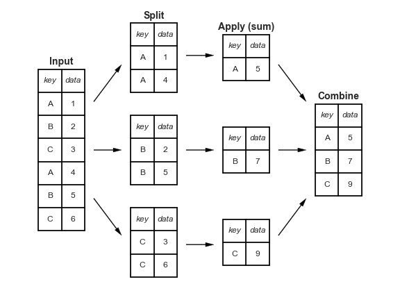
Grouping and Summarizing Data

Operations:

  • Grouping data by specific variables/column indices
  • Summarize/aggregate data by specific group features

group by

In [40]:
# Pandas: group by a column entries. 

# Generates an iterable where each group is broken up into a tuple (group,data).
# We can iterate across the tuple positions. 
g = dat.groupby(["continent"])
g
Out[40]:
<pandas.core.groupby.groupby.DataFrameGroupBy object at 0x7fb3289a8940>
In [41]:
for i in g:
    print(i[0],i[1].head(2))
Africa     country continent  year  lifeExp  population    gdpPercap  lifeExp_std
24  Algeria    Africa  1952   43.077     9279525  2449.008185    38.472684
25  Algeria    Africa  1957   45.685    10270856  3013.976023    41.080684
Americas       country continent  year  lifeExp  population    gdpPercap  lifeExp_std
48  Argentina  Americas  1952   62.485    17876956  5911.315053    57.880684
49  Argentina  Americas  1957   64.399    19610538  6856.856212    59.794684
Asia        country continent  year  lifeExp  population   gdpPercap  lifeExp_std
0  Afghanistan      Asia  1952   28.801     8425333  779.445314    24.196684
1  Afghanistan      Asia  1957   30.332     9240934  820.853030    25.727684
Europe     country continent  year  lifeExp  population    gdpPercap  lifeExp_std
12  Albania    Europe  1952    55.23     1282697  1601.056136    50.625684
13  Albania    Europe  1957    59.28     1476505  1942.284244    54.675684
Oceania       country continent  year  lifeExp  population    gdpPercap  lifeExp_std
60  Australia   Oceania  1952    69.12     8691212  10039.59564    64.515684
61  Australia   Oceania  1957    70.33     9712569  10949.64959    65.725684
In [42]:
dat.groupby(["continent"]).head(2)
Out[42]:
country continent year lifeExp population gdpPercap lifeExp_std
0 Afghanistan Asia 1952 28.801 8425333 779.445314 24.196684
1 Afghanistan Asia 1957 30.332 9240934 820.853030 25.727684
12 Albania Europe 1952 55.230 1282697 1601.056136 50.625684
13 Albania Europe 1957 59.280 1476505 1942.284244 54.675684
24 Algeria Africa 1952 43.077 9279525 2449.008185 38.472684
25 Algeria Africa 1957 45.685 10270856 3013.976023 41.080684
48 Argentina Americas 1952 62.485 17876956 5911.315053 57.880684
49 Argentina Americas 1957 64.399 19610538 6856.856212 59.794684
60 Australia Oceania 1952 69.120 8691212 10039.595640 64.515684
61 Australia Oceania 1957 70.330 9712569 10949.649590 65.725684
In [43]:
# dfply: group by a column entries. 
dat >> group_by(X.continent) >> head(2)
Out[43]:
country continent year lifeExp population gdpPercap lifeExp_std
24 Algeria Africa 1952 43.077 9279525 2449.008185 38.472684
25 Algeria Africa 1957 45.685 10270856 3013.976023 41.080684
48 Argentina Americas 1952 62.485 17876956 5911.315053 57.880684
49 Argentina Americas 1957 64.399 19610538 6856.856212 59.794684
0 Afghanistan Asia 1952 28.801 8425333 779.445314 24.196684
1 Afghanistan Asia 1957 30.332 9240934 820.853030 25.727684
12 Albania Europe 1952 55.230 1282697 1601.056136 50.625684
13 Albania Europe 1957 59.280 1476505 1942.284244 54.675684
60 Australia Oceania 1952 69.120 8691212 10039.595640 64.515684
61 Australia Oceania 1957 70.330 9712569 10949.649590 65.725684

With dfply, the group_by() method will persist. As we need to ungroup() if we wish to turn off the key.

In [44]:
d = dat >> group_by(X.continent) 
d >> head(2)
Out[44]:
country continent year lifeExp population gdpPercap lifeExp_std
24 Algeria Africa 1952 43.077 9279525 2449.008185 38.472684
25 Algeria Africa 1957 45.685 10270856 3013.976023 41.080684
48 Argentina Americas 1952 62.485 17876956 5911.315053 57.880684
49 Argentina Americas 1957 64.399 19610538 6856.856212 59.794684
0 Afghanistan Asia 1952 28.801 8425333 779.445314 24.196684
1 Afghanistan Asia 1957 30.332 9240934 820.853030 25.727684
12 Albania Europe 1952 55.230 1282697 1601.056136 50.625684
13 Albania Europe 1957 59.280 1476505 1942.284244 54.675684
60 Australia Oceania 1952 69.120 8691212 10039.595640 64.515684
61 Australia Oceania 1957 70.330 9712569 10949.649590 65.725684
In [45]:
d >> ungroup() >> head(2)
Out[45]:
country continent year lifeExp population gdpPercap lifeExp_std
0 Afghanistan Asia 1952 28.801 8425333 779.445314 24.196684
1 Afghanistan Asia 1957 30.332 9240934 820.853030 25.727684

Summarize

The power of a grouping function (like .groupby() shines when coupled with an aggregation operation.

From Python Data Science Handbook by Jake VanderPlas

pandas: .groupby() + .aggregate()

In [46]:
dat.groupby(["continent"]).mean()
Out[46]:
year lifeExp population gdpPercap lifeExp_std
continent
Africa 1979.5 48.865330 9.916003e+06 2193.754578 44.261015
Americas 1979.5 64.658737 2.450479e+07 7136.110356 60.054421
Asia 1979.5 60.064903 7.703872e+07 7902.150428 55.460588
Europe 1979.5 71.903686 1.716976e+07 14469.475533 67.299370
Oceania 1979.5 74.326208 8.874672e+06 18621.609223 69.721893

or select a specific variable to perform the aggregation step on.

In [47]:
dat.groupby(['continent'])[['lifeExp','gdpPercap']].mean()
Out[47]:
lifeExp gdpPercap
continent
Africa 48.865330 2193.754578
Americas 64.658737 7136.110356
Asia 60.064903 7902.150428
Europe 71.903686 14469.475533
Oceania 74.326208 18621.609223

Alternatively, we can specify a whole range of operations to aggregate by (along with specific variable columns) using the .aggregate()/.agg() method. To keep track of which operations correspond which variable, pandas will generate a hierarchical index for column entries.

In [48]:
dat.groupby(['continent'])[['lifeExp','gdpPercap']].agg(["mean","std","median"])
Out[48]:
lifeExp gdpPercap
mean std median mean std median
continent
Africa 48.865330 9.150210 47.7920 2193.754578 2827.929863 1192.138217
Americas 64.658737 9.345088 67.0480 7136.110356 6396.764112 5465.509853
Asia 60.064903 11.864532 61.7915 7902.150428 14045.373112 2646.786844
Europe 71.903686 5.433178 72.2410 14469.475533 9355.213498 12081.749115
Oceania 74.326208 3.795611 73.6650 18621.609223 6358.983321 17983.303955

Note that we can feed in user-defined functions into the aggregate() function as well.

In [49]:
def mean_add_50(x):
    return np.mean(x) + 50

dat.groupby(['continent'])[['lifeExp','gdpPercap']].agg(["mean","std","median",mean_add_50])
Out[49]:
lifeExp gdpPercap
mean std median mean_add_50 mean std median mean_add_50
continent
Africa 48.865330 9.150210 47.7920 98.865330 2193.754578 2827.929863 1192.138217 2243.754578
Americas 64.658737 9.345088 67.0480 114.658737 7136.110356 6396.764112 5465.509853 7186.110356
Asia 60.064903 11.864532 61.7915 110.064903 7902.150428 14045.373112 2646.786844 7952.150428
Europe 71.903686 5.433178 72.2410 121.903686 14469.475533 9355.213498 12081.749115 14519.475533
Oceania 74.326208 3.795611 73.6650 124.326208 18621.609223 6358.983321 17983.303955 18671.609223

If greater control over which indicators received which aggregation operation is required, one can provide a dictionary of variable and operation pairs.

In [50]:
dat.groupby(['continent']).agg({"lifeExp":"mean","gdpPercap":mean_add_50})
Out[50]:
lifeExp gdpPercap
continent
Africa 48.865330 2243.754578
Americas 64.658737 7186.110356
Asia 60.064903 7952.150428
Europe 71.903686 14519.475533
Oceania 74.326208 18671.609223

Finally we can group by more than one variable (i.e. implement a multi-index on the rows).

In [51]:
dat.groupby(['continent','country'])[['lifeExp','gdpPercap']].mean()
Out[51]:
lifeExp gdpPercap
continent country
Africa Algeria 59.030167 4426.025973
Angola 37.883500 3607.100529
Benin 48.779917 1155.395107
Botswana 54.597500 5031.503557
Burkina Faso 44.694000 843.990665
Burundi 44.817333 471.662990
Cameroon 48.128500 1774.634222
Central African Republic 43.866917 958.784697
Chad 46.773583 1165.453674
Comoros 52.381750 1314.380339
Congo, Dem. Rep. 44.543750 648.342646
Congo, Rep. 52.501917 3312.788215
Cote d'Ivoire 48.436167 1912.825382
Djibouti 46.380750 2697.833162
Egypt 56.243000 3074.030731
Equatorial Guinea 42.960000 2469.166681
Eritrea 45.999250 541.002507
Ethiopia 44.475750 509.115155
Gabon 51.220500 11529.865474
Gambia 44.400583 680.132586
Ghana 52.340667 1044.582046
Guinea 43.239833 776.067305
Guinea-Bissau 39.210250 652.157208
Kenya 52.681000 1200.415720
Lesotho 50.007083 780.553393
Liberia 42.476250 604.814141
Libya 59.304167 12013.579201
Madagascar 47.770583 1335.595027
Malawi 43.351583 575.447212
Mali 43.413500 673.093069
... ... ... ...
Europe Belgium 73.641750 19900.758072
Bosnia and Herzegovina 67.707833 3484.779069
Bulgaria 69.743750 6384.055172
Croatia 70.055917 9331.712346
Czech Republic 71.510500 13920.011379
Denmark 74.370167 21671.824888
Finland 72.991917 17473.722667
France 74.348917 18833.570327
Germany 73.444417 20556.684433
Greece 73.733167 13969.036833
Hungary 69.393167 10888.175654
Iceland 76.511417 20531.422272
Ireland 73.017250 15758.606238
Italy 74.013833 16245.209006
Montenegro 70.299167 7208.064560
Netherlands 75.648500 21748.852208
Norway 75.843000 26747.306554
Poland 70.176917 8416.553912
Portugal 70.419833 11354.091927
Romania 68.290667 7300.169974
Serbia 68.551000 9305.049444
Slovak Republic 70.696083 10415.530689
Slovenia 71.600750 14074.582109
Spain 74.203417 14029.826479
Sweden 76.177000 19943.126104
Switzerland 75.565083 27074.334405
Turkey 59.696417 4469.453380
United Kingdom 73.922583 19380.472986
Oceania Australia 74.662917 19980.595634
New Zealand 73.989500 17262.622813

142 rows × 2 columns

dfply: group_by() + summarize()

We can emulate much the same behavior with the group_by() and summarize() methods.

In [52]:
dat >> group_by(X.continent) >> summarize(lifeExp_mean = X.lifeExp.mean(),
                                          lifeExp_std = X.lifeExp.std(),
                                          lifeExp_mean50 = mean_add_50(X.lifeExp))
Out[52]:
continent lifeExp_mean lifeExp_std lifeExp_mean50
0 Africa 48.865330 9.150210 98.865330
1 Americas 64.658737 9.345088 114.658737
2 Asia 60.064903 11.864532 110.064903
3 Europe 71.903686 5.433178 121.903686
4 Oceania 74.326208 3.795611 124.326208

dfply: group_by() + summarize_each()

In [53]:
dat >> group_by(X.continent) >> summarize_each([np.mean,np.std,mean_add_50],X.lifeExp,X.gdpPercap)
Out[53]:
continent lifeExp_mean lifeExp_std lifeExp_mean_add_50 gdpPercap_mean gdpPercap_std gdpPercap_mean_add_50
0 Africa 48.865330 9.142875 98.865330 2193.754578 2825.662985 2243.754578
1 Americas 64.658737 9.329500 114.658737 7136.110356 6386.093939 7186.110356
2 Asia 60.064903 11.849542 110.064903 7902.150428 14027.627845 7952.150428
3 Europe 71.903686 5.425626 121.903686 14469.475533 9342.211111 14519.475533
4 Oceania 74.326208 3.715695 124.326208 18621.609223 6225.094993 18671.609223

Transforming and Applying

Other times we want to implement data manipulations by some grouping variable but retain structure of the original data. Put differently, our aim is not to aggregate but to perform some operation across specific groups. For example, we might want to group-mean center our variables as a way of removing between group variation.

In [54]:
# Pandas: groupby() + transform()
def center(x):
    '''Center a variable around its mean'''
    return x - x.mean()

dat.groupby('country')[["lifeExp","population"]].transform(center).head(10)
Out[54]:
lifeExp population
0 -8.677833 -7.398382e+06
1 -7.146833 -6.582781e+06
2 -5.481833 -5.556632e+06
3 -3.458833 -4.285749e+06
4 -1.390833 -2.744255e+06
5 0.959167 -9.433434e+05
6 2.375167 -2.941899e+06
7 3.343167 -1.955758e+06
8 4.195167 4.942056e+05
9 4.284167 6.403700e+06

Likewise, apply() offers identical functionality. The only requirement of apply is that the output must be a pandas.DataFrame, a pandas.Series, or a scalar.

In [55]:
# Pandas: groupby() + apply()
dat.groupby('country')[["lifeExp","population"]].apply(center).head(10)
Out[55]:
lifeExp population
0 -8.677833 -7.398382e+06
1 -7.146833 -6.582781e+06
2 -5.481833 -5.556632e+06
3 -3.458833 -4.285749e+06
4 -1.390833 -2.744255e+06
5 0.959167 -9.433434e+05
6 2.375167 -2.941899e+06
7 3.343167 -1.955758e+06
8 4.195167 4.942056e+05
9 4.284167 6.403700e+06
In [56]:
# dfply: group_by + mutate()
d = dat >> group_by(X.country) >> mutate(lifeExp_centered = center(X.lifeExp),
                                         population_centered = center(X.population)) 
d.head(10)
Out[56]:
country continent year lifeExp population gdpPercap lifeExp_std lifeExp_centered population_centered
0 Afghanistan Asia 1952 28.801 8425333 779.445314 24.196684 -8.677833 -7.398382e+06
1 Afghanistan Asia 1957 30.332 9240934 820.853030 25.727684 -7.146833 -6.582781e+06
2 Afghanistan Asia 1962 31.997 10267083 853.100710 27.392684 -5.481833 -5.556632e+06
3 Afghanistan Asia 1967 34.020 11537966 836.197138 29.415684 -3.458833 -4.285749e+06
4 Afghanistan Asia 1972 36.088 13079460 739.981106 31.483684 -1.390833 -2.744255e+06
5 Afghanistan Asia 1977 38.438 14880372 786.113360 33.833684 0.959167 -9.433434e+05
6 Afghanistan Asia 1982 39.854 12881816 978.011439 35.249684 2.375167 -2.941899e+06
7 Afghanistan Asia 1987 40.822 13867957 852.395945 36.217684 3.343167 -1.955758e+06
8 Afghanistan Asia 1992 41.674 16317921 649.341395 37.069684 4.195167 4.942056e+05
9 Afghanistan Asia 1997 41.763 22227415 635.341351 37.158684 4.284167 6.403700e+06

To emulate pandas and just return the transformed columns, we can use transmute() which is identical to mutate() but only return the changed variables

In [57]:
d = dat >> group_by(X.country) >> transmute(lifeExp_centered = center(X.lifeExp),
                                            population_centered = center(X.population)) 
d.head(10)
Out[57]:
country lifeExp_centered population_centered
0 Afghanistan -8.677833 -7.398382e+06
1 Afghanistan -7.146833 -6.582781e+06
2 Afghanistan -5.481833 -5.556632e+06
3 Afghanistan -3.458833 -4.285749e+06
4 Afghanistan -1.390833 -2.744255e+06
5 Afghanistan 0.959167 -9.433434e+05
6 Afghanistan 2.375167 -2.941899e+06
7 Afghanistan 3.343167 -1.955758e+06
8 Afghanistan 4.195167 4.942056e+05
9 Afghanistan 4.284167 6.403700e+06

Reshaping and Reordering Data

Operations:

  • Sorting values by variables/column indices
  • Altering the shape of a data construct: wide-to-long and vice versa

Sorting values

In [58]:
# Pandas: sort values by a column variable (ascending)
dat.sort_values('country').head(3)
Out[58]:
country continent year lifeExp population gdpPercap lifeExp_std
0 Afghanistan Asia 1952 28.801 8425333 779.445314 24.196684
11 Afghanistan Asia 2007 43.828 31889923 974.580338 39.223684
10 Afghanistan Asia 2002 42.129 25268405 726.734055 37.524684
In [59]:
# Pandas: sort values by a column variable (descending)
dat.sort_values('country',ascending=False).head(3)
Out[59]:
country continent year lifeExp population gdpPercap lifeExp_std
1703 Zimbabwe Africa 2007 43.487 12311143 469.709298 38.882684
1697 Zimbabwe Africa 1977 57.674 6642107 685.587682 53.069684
1692 Zimbabwe Africa 1952 48.451 3080907 406.884115 43.846684
In [60]:
# Pandas: sort values by more than one column variable 
dat.sort_values(['country','year'],ascending=False).head(3)
Out[60]:
country continent year lifeExp population gdpPercap lifeExp_std
1703 Zimbabwe Africa 2007 43.487 12311143 469.709298 38.882684
1702 Zimbabwe Africa 2002 39.989 11926563 672.038623 35.384684
1701 Zimbabwe Africa 1997 46.809 11404948 792.449960 42.204684
In [61]:
# dfply: sort values by a column variable (ascending)
dat >> arrange(X.country) >> head(3)
Out[61]:
country continent year lifeExp population gdpPercap lifeExp_std
0 Afghanistan Asia 1952 28.801 8425333 779.445314 24.196684
11 Afghanistan Asia 2007 43.828 31889923 974.580338 39.223684
10 Afghanistan Asia 2002 42.129 25268405 726.734055 37.524684
In [62]:
# dfply: sort values by a column variable (descending)
dat >> arrange(desc(X.country)) >> head(3)
Out[62]:
country continent year lifeExp population gdpPercap lifeExp_std
1703 Zimbabwe Africa 2007 43.487 12311143 469.709298 38.882684
1692 Zimbabwe Africa 1952 48.451 3080907 406.884115 43.846684
1693 Zimbabwe Africa 1957 50.469 3646340 518.764268 45.864684
In [63]:
# dfply: sort values by more than one column variable 
dat >> arrange(desc(X.country),X.year) >> head(3)
Out[63]:
country continent year lifeExp population gdpPercap lifeExp_std
1692 Zimbabwe Africa 1952 48.451 3080907 406.884115 43.846684
1693 Zimbabwe Africa 1957 50.469 3646340 518.764268 45.864684
1694 Zimbabwe Africa 1962 52.358 4277736 527.272182 47.753684

Reshaping Data

long-to-wide

In [64]:
# pandas: long to wide using the pivot_table() method
dat.pivot_table('gdpPercap', index='year', columns='country')
Out[64]:
country Afghanistan Albania Algeria Angola Argentina Australia Austria Bahrain Bangladesh Belgium ... Uganda United Kingdom United States Uruguay Venezuela Vietnam West Bank and Gaza Yemen, Rep. Zambia Zimbabwe
year
1952 779.445314 1601.056136 2449.008185 3520.610273 5911.315053 10039.59564 6137.076492 9867.084765 684.244172 8343.105127 ... 734.753484 9979.508487 13990.48208 5716.766744 7689.799761 605.066492 1515.592329 781.717576 1147.388831 406.884115
1957 820.853030 1942.284244 3013.976023 3827.940465 6856.856212 10949.64959 8842.598030 11635.799450 661.637458 9714.960623 ... 774.371069 11283.177950 14847.12712 6150.772969 9802.466526 676.285448 1827.067742 804.830455 1311.956766 518.764268
1962 853.100710 2312.888958 2550.816880 4269.276742 7133.166023 12217.22686 10750.721110 12753.275140 686.341554 10991.206760 ... 767.271740 12477.177070 16173.14586 5603.357717 8422.974165 772.049160 2198.956312 825.623201 1452.725766 527.272182
1967 836.197138 2760.196931 3246.991771 5522.776375 8052.953021 14526.12465 12834.602400 14804.672700 721.186086 13149.041190 ... 908.918522 14142.850890 19530.36557 5444.619620 9541.474188 637.123289 2649.715007 862.442146 1777.077318 569.795071
1972 739.981106 3313.422188 4182.663766 5473.288005 9443.038526 16788.62948 16661.625600 18268.658390 630.233627 16672.143560 ... 950.735869 15895.116410 21806.03594 5703.408898 10505.259660 699.501644 3133.409277 1265.047031 1773.498265 799.362176
1977 786.113360 3533.003910 4910.416756 3008.647355 10079.026740 18334.19751 19749.422300 19340.101960 659.877232 19117.974480 ... 843.733137 17428.748460 24072.63213 6504.339663 13143.950950 713.537120 3682.831494 1829.765177 1588.688299 685.587682
1982 978.011439 3630.880722 5745.160213 2756.953672 8997.897412 19477.00928 21597.083620 19211.147310 676.981866 20979.845890 ... 682.266227 18232.424520 25009.55914 6920.223051 11152.410110 707.235786 4336.032082 1977.557010 1408.678565 788.855041
1987 852.395945 3738.932735 5681.358539 2430.208311 9139.671389 21888.88903 23687.826070 18524.024060 751.979403 22525.563080 ... 617.724406 21664.787670 29884.35041 7452.398969 9883.584648 820.799445 5107.197384 1971.741538 1213.315116 706.157306
1992 649.341395 2497.437901 5023.216647 2627.845685 9308.418710 23424.76683 27042.018680 19035.579170 837.810164 25575.570690 ... 644.170797 22705.092540 32003.93224 8137.004775 10733.926310 989.023149 6017.654756 1879.496673 1210.884633 693.420786
1997 635.341351 3193.054604 4797.295051 2277.140884 10967.281950 26997.93657 29095.920660 20292.016790 972.770035 27561.196630 ... 816.559081 26074.531360 35767.43303 9230.240708 10165.495180 1385.896769 7110.667619 2117.484526 1071.353818 792.449960
2002 726.734055 4604.211737 5288.040382 2773.287312 8797.640716 30687.75473 32417.607690 23403.559270 1136.390430 30485.883750 ... 927.721002 29478.999190 39097.09955 7727.002004 8605.047831 1764.456677 4515.487575 2234.820827 1071.613938 672.038623
2007 974.580338 5937.029526 6223.367465 4797.231267 12779.379640 34435.36744 36126.492700 29796.048340 1391.253792 33692.605080 ... 1056.380121 33203.261280 42951.65309 10611.462990 11415.805690 2441.576404 3025.349798 2280.769906 1271.211593 469.709298

12 rows × 142 columns

In [65]:
# Recall we can emulate the same pivoting behavior using 
# by resetting the index and unstacking
dat.set_index(["country","year"])['gdpPercap'].unstack(level="country")
Out[65]:
country Afghanistan Albania Algeria Angola Argentina Australia Austria Bahrain Bangladesh Belgium ... Uganda United Kingdom United States Uruguay Venezuela Vietnam West Bank and Gaza Yemen, Rep. Zambia Zimbabwe
year
1952 779.445314 1601.056136 2449.008185 3520.610273 5911.315053 10039.59564 6137.076492 9867.084765 684.244172 8343.105127 ... 734.753484 9979.508487 13990.48208 5716.766744 7689.799761 605.066492 1515.592329 781.717576 1147.388831 406.884115
1957 820.853030 1942.284244 3013.976023 3827.940465 6856.856212 10949.64959 8842.598030 11635.799450 661.637458 9714.960623 ... 774.371069 11283.177950 14847.12712 6150.772969 9802.466526 676.285448 1827.067742 804.830455 1311.956766 518.764268
1962 853.100710 2312.888958 2550.816880 4269.276742 7133.166023 12217.22686 10750.721110 12753.275140 686.341554 10991.206760 ... 767.271740 12477.177070 16173.14586 5603.357717 8422.974165 772.049160 2198.956312 825.623201 1452.725766 527.272182
1967 836.197138 2760.196931 3246.991771 5522.776375 8052.953021 14526.12465 12834.602400 14804.672700 721.186086 13149.041190 ... 908.918522 14142.850890 19530.36557 5444.619620 9541.474188 637.123289 2649.715007 862.442146 1777.077318 569.795071
1972 739.981106 3313.422188 4182.663766 5473.288005 9443.038526 16788.62948 16661.625600 18268.658390 630.233627 16672.143560 ... 950.735869 15895.116410 21806.03594 5703.408898 10505.259660 699.501644 3133.409277 1265.047031 1773.498265 799.362176
1977 786.113360 3533.003910 4910.416756 3008.647355 10079.026740 18334.19751 19749.422300 19340.101960 659.877232 19117.974480 ... 843.733137 17428.748460 24072.63213 6504.339663 13143.950950 713.537120 3682.831494 1829.765177 1588.688299 685.587682
1982 978.011439 3630.880722 5745.160213 2756.953672 8997.897412 19477.00928 21597.083620 19211.147310 676.981866 20979.845890 ... 682.266227 18232.424520 25009.55914 6920.223051 11152.410110 707.235786 4336.032082 1977.557010 1408.678565 788.855041
1987 852.395945 3738.932735 5681.358539 2430.208311 9139.671389 21888.88903 23687.826070 18524.024060 751.979403 22525.563080 ... 617.724406 21664.787670 29884.35041 7452.398969 9883.584648 820.799445 5107.197384 1971.741538 1213.315116 706.157306
1992 649.341395 2497.437901 5023.216647 2627.845685 9308.418710 23424.76683 27042.018680 19035.579170 837.810164 25575.570690 ... 644.170797 22705.092540 32003.93224 8137.004775 10733.926310 989.023149 6017.654756 1879.496673 1210.884633 693.420786
1997 635.341351 3193.054604 4797.295051 2277.140884 10967.281950 26997.93657 29095.920660 20292.016790 972.770035 27561.196630 ... 816.559081 26074.531360 35767.43303 9230.240708 10165.495180 1385.896769 7110.667619 2117.484526 1071.353818 792.449960
2002 726.734055 4604.211737 5288.040382 2773.287312 8797.640716 30687.75473 32417.607690 23403.559270 1136.390430 30485.883750 ... 927.721002 29478.999190 39097.09955 7727.002004 8605.047831 1764.456677 4515.487575 2234.820827 1071.613938 672.038623
2007 974.580338 5937.029526 6223.367465 4797.231267 12779.379640 34435.36744 36126.492700 29796.048340 1391.253792 33692.605080 ... 1056.380121 33203.261280 42951.65309 10611.462990 11415.805690 2441.576404 3025.349798 2280.769906 1271.211593 469.709298

12 rows × 142 columns

.pivot_table() also allows for us to feed in an aggregation function among other arguments.

In [66]:
dat.pivot_table(index=['continent','year'],columns=['country'],
               aggfunc='mean',fill_value=-99).head(10)
Out[66]:
gdpPercap ... population
country Afghanistan Albania Algeria Angola Argentina Australia Austria Bahrain Bangladesh Belgium ... Uganda United Kingdom United States Uruguay Venezuela Vietnam West Bank and Gaza Yemen, Rep. Zambia Zimbabwe
continent year
Africa 1952 -99.0 -99.0 2449.008185 3520.610273 -99.0 -99.0 -99.0 -99.0 -99.0 -99.0 ... 5824797 -99 -99 -99 -99 -99 -99 -99 2672000 3080907
1957 -99.0 -99.0 3013.976023 3827.940465 -99.0 -99.0 -99.0 -99.0 -99.0 -99.0 ... 6675501 -99 -99 -99 -99 -99 -99 -99 3016000 3646340
1962 -99.0 -99.0 2550.816880 4269.276742 -99.0 -99.0 -99.0 -99.0 -99.0 -99.0 ... 7688797 -99 -99 -99 -99 -99 -99 -99 3421000 4277736
1967 -99.0 -99.0 3246.991771 5522.776375 -99.0 -99.0 -99.0 -99.0 -99.0 -99.0 ... 8900294 -99 -99 -99 -99 -99 -99 -99 3900000 4995432
1972 -99.0 -99.0 4182.663766 5473.288005 -99.0 -99.0 -99.0 -99.0 -99.0 -99.0 ... 10190285 -99 -99 -99 -99 -99 -99 -99 4506497 5861135
1977 -99.0 -99.0 4910.416756 3008.647355 -99.0 -99.0 -99.0 -99.0 -99.0 -99.0 ... 11457758 -99 -99 -99 -99 -99 -99 -99 5216550 6642107
1982 -99.0 -99.0 5745.160213 2756.953672 -99.0 -99.0 -99.0 -99.0 -99.0 -99.0 ... 12939400 -99 -99 -99 -99 -99 -99 -99 6100407 7636524
1987 -99.0 -99.0 5681.358539 2430.208311 -99.0 -99.0 -99.0 -99.0 -99.0 -99.0 ... 15283050 -99 -99 -99 -99 -99 -99 -99 7272406 9216418
1992 -99.0 -99.0 5023.216647 2627.845685 -99.0 -99.0 -99.0 -99.0 -99.0 -99.0 ... 18252190 -99 -99 -99 -99 -99 -99 -99 8381163 10704340
1997 -99.0 -99.0 4797.295051 2277.140884 -99.0 -99.0 -99.0 -99.0 -99.0 -99.0 ... 21210254 -99 -99 -99 -99 -99 -99 -99 9417789 11404948

10 rows × 568 columns

In [67]:
# dfply: long to wide using the spread() method
# We want to feed the spread function a columns position and a value postion.

dat >> select(X.country,X.year,X.gdpPercap) >> spread(X.country,X.gdpPercap)
Out[67]:
year Afghanistan Albania Algeria Angola Argentina Australia Austria Bahrain Bangladesh ... Uganda United Kingdom United States Uruguay Venezuela Vietnam West Bank and Gaza Yemen, Rep. Zambia Zimbabwe
0 1952 779.445314 1601.056136 2449.008185 3520.610273 5911.315053 10039.59564 6137.076492 9867.084765 684.244172 ... 734.753484 9979.508487 13990.48208 5716.766744 7689.799761 605.066492 1515.592329 781.717576 1147.388831 406.884115
1 1957 820.853030 1942.284244 3013.976023 3827.940465 6856.856212 10949.64959 8842.598030 11635.799450 661.637458 ... 774.371069 11283.177950 14847.12712 6150.772969 9802.466526 676.285448 1827.067742 804.830455 1311.956766 518.764268
2 1962 853.100710 2312.888958 2550.816880 4269.276742 7133.166023 12217.22686 10750.721110 12753.275140 686.341554 ... 767.271740 12477.177070 16173.14586 5603.357717 8422.974165 772.049160 2198.956312 825.623201 1452.725766 527.272182
3 1967 836.197138 2760.196931 3246.991771 5522.776375 8052.953021 14526.12465 12834.602400 14804.672700 721.186086 ... 908.918522 14142.850890 19530.36557 5444.619620 9541.474188 637.123289 2649.715007 862.442146 1777.077318 569.795071
4 1972 739.981106 3313.422188 4182.663766 5473.288005 9443.038526 16788.62948 16661.625600 18268.658390 630.233627 ... 950.735869 15895.116410 21806.03594 5703.408898 10505.259660 699.501644 3133.409277 1265.047031 1773.498265 799.362176
5 1977 786.113360 3533.003910 4910.416756 3008.647355 10079.026740 18334.19751 19749.422300 19340.101960 659.877232 ... 843.733137 17428.748460 24072.63213 6504.339663 13143.950950 713.537120 3682.831494 1829.765177 1588.688299 685.587682
6 1982 978.011439 3630.880722 5745.160213 2756.953672 8997.897412 19477.00928 21597.083620 19211.147310 676.981866 ... 682.266227 18232.424520 25009.55914 6920.223051 11152.410110 707.235786 4336.032082 1977.557010 1408.678565 788.855041
7 1987 852.395945 3738.932735 5681.358539 2430.208311 9139.671389 21888.88903 23687.826070 18524.024060 751.979403 ... 617.724406 21664.787670 29884.35041 7452.398969 9883.584648 820.799445 5107.197384 1971.741538 1213.315116 706.157306
8 1992 649.341395 2497.437901 5023.216647 2627.845685 9308.418710 23424.76683 27042.018680 19035.579170 837.810164 ... 644.170797 22705.092540 32003.93224 8137.004775 10733.926310 989.023149 6017.654756 1879.496673 1210.884633 693.420786
9 1997 635.341351 3193.054604 4797.295051 2277.140884 10967.281950 26997.93657 29095.920660 20292.016790 972.770035 ... 816.559081 26074.531360 35767.43303 9230.240708 10165.495180 1385.896769 7110.667619 2117.484526 1071.353818 792.449960
10 2002 726.734055 4604.211737 5288.040382 2773.287312 8797.640716 30687.75473 32417.607690 23403.559270 1136.390430 ... 927.721002 29478.999190 39097.09955 7727.002004 8605.047831 1764.456677 4515.487575 2234.820827 1071.613938 672.038623
11 2007 974.580338 5937.029526 6223.367465 4797.231267 12779.379640 34435.36744 36126.492700 29796.048340 1391.253792 ... 1056.380121 33203.261280 42951.65309 10611.462990 11415.805690 2441.576404 3025.349798 2280.769906 1271.211593 469.709298

12 rows × 143 columns

wide-to-long

In [68]:
# Pandas: wide-to-long using the melt method
pd.melt(dat,id_vars=['country','continent','year']).head()
Out[68]:
country continent year variable value
0 Afghanistan Asia 1952 lifeExp 28.801
1 Afghanistan Asia 1957 lifeExp 30.332
2 Afghanistan Asia 1962 lifeExp 31.997
3 Afghanistan Asia 1967 lifeExp 34.020
4 Afghanistan Asia 1972 lifeExp 36.088
In [69]:
# Recall that we can emulate this behavior with the set_index and stack methods
dat.set_index(['country','continent','year']).stack().head()
Out[69]:
country      continent  year             
Afghanistan  Asia       1952  lifeExp        2.880100e+01
                              population     8.425333e+06
                              gdpPercap      7.794453e+02
                              lifeExp_std    2.419668e+01
                        1957  lifeExp        3.033200e+01
dtype: float64
In [70]:
# dfply: wide-to-long using the gather method
dat >> gather('variable', 'value',["lifeExp",'gdpPercap','population','lifeExp_std']) >> head()
Out[70]:
country continent year variable value
0 Afghanistan Asia 1952 lifeExp 28.801
1 Afghanistan Asia 1957 lifeExp 30.332
2 Afghanistan Asia 1962 lifeExp 31.997
3 Afghanistan Asia 1967 lifeExp 34.020
4 Afghanistan Asia 1972 lifeExp 36.088

Piping

Operations:

  • Chain together data manipulations in a single operational sequence.

These are powerful operations in isolation, but when combined, what results is a streamlined way to convert raw data into a useful data construct. We can do this because pandas was built fully utilizing a fluid programming framework (that is, the class always returns itself after every call).

This is easier to show in practice. Let's consider different ways to perform the same sequence of operations.

Let's do the following: Aggregate the data to the country level for all countries in Asia

Method 1: sequentially overwrite the object

In [71]:
dat = pd.read_csv("gapminder.csv") # Read the data in

dat = dat.query("continent == 'Asia'")
dat = dat.filter(['country','lifeExp','gdpPercap','population'])
dat = dat.groupby(['country'])
dat = dat.agg(mean)
dat = dat.reset_index()

dat.round(1).head()
Out[71]:
country lifeExp gdpPercap population
0 Afghanistan 37.5 802.7 15823715.4
1 Bahrain 65.6 18077.7 373913.2
2 Bangladesh 49.8 817.6 90755395.3
3 Cambodia 47.9 675.4 8510430.7
4 China 61.8 1488.3 958160051.9
In [72]:
dat = pd.read_csv("gapminder.csv")

dat = dat.query("continent == 'Asia'").filter(['country','lifeExp','gdpPercap','population']).groupby(['country']).agg(mean).reset_index()

dat.round(1).head()
Out[72]:
country lifeExp gdpPercap population
0 Afghanistan 37.5 802.7 15823715.4
1 Bahrain 65.6 18077.7 373913.2
2 Bangladesh 49.8 817.6 90755395.3
3 Cambodia 47.9 675.4 8510430.7
4 China 61.8 1488.3 958160051.9

Method 3: Do it all in one step by piping

In [73]:
dat = pd.read_csv("gapminder.csv")

# (A) use the back slash
dat = dat.\
query("continent == 'Asia'").\
filter(['country','lifeExp','gdpPercap','population']).\
groupby(['country']).\
agg(mean).\
reset_index()

dat.round(1).head()
Out[73]:
country lifeExp gdpPercap population
0 Afghanistan 37.5 802.7 15823715.4
1 Bahrain 65.6 18077.7 373913.2
2 Bangladesh 49.8 817.6 90755395.3
3 Cambodia 47.9 675.4 8510430.7
4 China 61.8 1488.3 958160051.9
In [74]:
dat = pd.read_csv("gapminder.csv")

# (B) house in parentheses
dat = (dat
       .query("continent == 'Asia'")
       .filter(['country','lifeExp','gdpPercap','population'])
       .groupby(['country'])
       .agg(mean)
       .reset_index())

dat.round(1).head()
Out[74]:
country lifeExp gdpPercap population
0 Afghanistan 37.5 802.7 15823715.4
1 Bahrain 65.6 18077.7 373913.2
2 Bangladesh 49.8 817.6 90755395.3
3 Cambodia 47.9 675.4 8510430.7
4 China 61.8 1488.3 958160051.9

piping with dfply

We've already seen this in play throughout the lecture notes.

In [108]:
dat = pd.read_csv("gapminder.csv")

dat = (dat >> 
       mask(X.continent == "Asia") >> 
       select(X.country,columns_between(X.lifeExp,X.gdpPercap)) >> 
       group_by(X.country) >>
       summarize_each([np.mean],X.lifeExp,X.gdpPercap,X.population))

dat.round(1).head()
Out[108]:
country lifeExp_mean gdpPercap_mean population_mean
0 Afghanistan 37.5 802.7 15823715.4
1 Bahrain 65.6 18077.7 373913.2
2 Bangladesh 49.8 817.6 90755395.3
3 Cambodia 47.9 675.4 8510430.7
4 China 61.8 1488.3 958160051.9

Miscellaneous

Views

Note that similar to numpy, we can manipulate a "view" of a pandas.DataFrame.

In [76]:
# Create a fake data frame
D = pd.DataFrame(dict(A=np.arange(5),
                     B=np.arange(5)*-1))
D
Out[76]:
A B
0 0 0
1 1 -1
2 2 -2
3 3 -3
4 4 -4
In [77]:
# Create and Manipulate a subset (view)
b = D.iloc[:2,:2]
b.iloc[:2,:2] = 8 
b
Out[77]:
A B
0 8 8
1 8 8
In [78]:
# Changes carry over to the original object
D
Out[78]:
A B
0 8 8
1 8 8
2 2 -2
3 3 -3
4 4 -4

Counting number of observations (by group)

In [79]:
dat = pd.read_csv("gapminder.csv")

# Pandas approach

# Country-Years
a = \
(dat
 .filter(["country"])
 .groupby(['country'])
 .size() # We can count the number of observations using the size method
 .reset_index()
 .rename(columns={0:"n_country_years"})
) 


# Countries by continent
b = \
(dat
 .filter(["continent","country"])
 .drop_duplicates()
 .groupby(['continent'])
 .size() # We can count the number of observations using the size method
 .reset_index()
 .rename(columns={0:"n_countries"})
 .head(5)
) 


# total countries  
c = \
(dat
 .filter(["country"])
 .drop_duplicates()
 .shape[0]
)


# Print
display(a.head(3))
display(b)
print(f'There are {c} total countries in the data.')
country n_country_years
0 Afghanistan 12
1 Albania 12
2 Algeria 12
continent n_countries
0 Africa 52
1 Americas 25
2 Asia 33
3 Europe 30
4 Oceania 2
There are 142 total countries in the data.
In [80]:
# dfply approach

# Country-Years
aa = \
(dat >> 
group_by(X.country) >> 
summarize(n_country_years = n(X.year)) >> 
head(3))

# Countries by continent
bb = \
(dat >> 
distinct(X.continent,X.country) >>
group_by(X.continent) >> 
summarize(n_countries = n(X.country)) >> 
head(3))

# total countries  
cc = dat >> summarize(n_total_countries = n_distinct(X.country))

# Print
display(aa.head(3))
display(bb)
display(cc)
country n_country_years
0 Afghanistan 12
1 Albania 12
2 Algeria 12
continent n_countries
0 Africa 52
1 Americas 25
2 Asia 33
3 Europe 30
4 Oceania 2
n_total_countries
0 142

Categories to dummies

In statistics and machine learning, we often need to convert a categorical variable into a dummy feature set (i.e. when the variable is "on" it takes the value of 1, 0 otherwise). In statistics, we'll use this type of conversion to generate fixed effects.

pandas makes this type of manipulation easy to do. with the

In [81]:
d = pd.DataFrame(dict(country = ["Nigeria","Nigeria","United States","United States","Russia","Russia"]))
d
Out[81]:
country
0 Nigeria
1 Nigeria
2 United States
3 United States
4 Russia
5 Russia
In [82]:
dummies = pd.get_dummies(d.country)
pd.concat([d,dummies],sort=False,axis=1)
Out[82]:
country Nigeria Russia United States
0 Nigeria 1 0 0
1 Nigeria 1 0 0
2 United States 0 0 1
3 United States 0 0 1
4 Russia 0 1 0
5 Russia 0 1 0

Merging with dfply

For the sake of completeness, let's demonstrate what joining looks like with dfply. Like dplyr (which the module is based off of), dfply uses SQl syntax to keep track of the type of merge we are performing.

In [83]:
# Same fake data construct as the prior lecture

data_A = pd.DataFrame(dict(country = ["Nigeria","England","Botswana"],
                           var1 = [4,3,6]))
data_B = pd.DataFrame(dict(country = ["Nigeria","United States","Botswana"],
                           var2 = ["low","high","medium"]))
display(data_A)
display(data_B)
country var1
0 Nigeria 4
1 England 3
2 Botswana 6
country var2
0 Nigeria low
1 United States high
2 Botswana medium
In [84]:
# Left Join
data_A >> left_join(data_B, by='country')
Out[84]:
country var1 var2
0 Nigeria 4 low
1 England 3 NaN
2 Botswana 6 medium
In [85]:
# right Join
data_A >> right_join(data_B, by='country')
Out[85]:
country var1 var2
0 Nigeria 4.0 low
1 Botswana 6.0 medium
2 United States NaN high
In [86]:
# Inner Join
data_A >> inner_join(data_B, by='country')
Out[86]:
country var1 var2
0 Nigeria 4 low
1 Botswana 6 medium
In [87]:
# Full Join
data_A >> full_join(data_B, by='country')
Out[87]:
country var1 var2
0 Nigeria 4.0 low
1 England 3.0 NaN
2 Botswana 6.0 medium
3 United States NaN high
In [88]:
# Or Outer Join (same as Full Join)
data_A >> outer_join(data_B, by='country')
Out[88]:
country var1 var2
0 Nigeria 4.0 low
1 England 3.0 NaN
2 Botswana 6.0 medium
3 United States NaN high
In [89]:
# Anti Join
data_A >> anti_join(data_B, by='country')
Out[89]:
country var1
1 England 3
In [90]:
# Bind Rows
data_A >> bind_rows(data_B)
/Library/Frameworks/Python.framework/Versions/3.7/lib/python3.7/site-packages/dfply/join.py:279: FutureWarning: Sorting because non-concatenation axis is not aligned. A future version
of pandas will change to not sort by default.

To accept the future behavior, pass 'sort=False'.

To retain the current behavior and silence the warning, pass 'sort=True'.

  df = pd.concat([df, other], join=join, ignore_index=ignore_index, axis=0)
Out[90]:
country var1 var2
0 Nigeria 4.0 NaN
1 England 3.0 NaN
2 Botswana 6.0 NaN
0 Nigeria NaN low
1 United States NaN high
2 Botswana NaN medium
In [91]:
# Bind columns
data_A >> bind_cols(data_B)
Out[91]:
country var1 country var2
0 Nigeria 4 Nigeria low
1 England 3 United States high
2 Botswana 6 Botswana medium