PPOL564 - Data Science I: Foundations

Lecture 8

Data Wrangling using Pandas

Part 1

Concepts Covered Today:

  • Overview of pandas data objects
  • Tidy data & indices
  • Import/Export/Conversions
  • Initial Exploration of Data Quality
  • Joining data
In [115]:
import pandas as pd
import numpy as np
import requests

Import data used in the notebook. Data will save to the notebook's directory

In [117]:
def download_data(git_loc,dest_name):
    '''
    Download data from Github and save to the notebook's working directory.
    '''
    req = requests.get(git_loc)
    with open(dest_name,"w") as file:
        for line in req.text:
            file.writelines(line)
            
download_data('https://raw.githubusercontent.com/edunford/ppol564/master/lectures/lecture_08/Data/StormEvents_details-ftp_v1.0_d1950_c20170120.csv',
         "storm_data.csv")
download_data('https://raw.githubusercontent.com/edunford/ppol564/master/lectures/lecture_08/Data/example_data.csv',
         "example_data.csv")

pandas Objects

Recall numpy offers a greater flexibility and efficiency when dealing with data matrices (when compared to manipulating data represented as a nested list). However, as we saw, numpy is limited in its capacity to deal with heterogeneous data types in a single data matrix. This is a limitation given the nature of most social science datasets.

The pandas package was designed to deal with this issue. Built on top of the numpy library, Pandas retains and expands upon numpy's functionality.

The fundamental data constructs in a pandas object is the Series and the DataFrame.

Series

A pandas series is a one-dimensional labeled array capable of holding heterogeneous data types (e.g. integer, boolean, strings, etc.). The axis in a series as "index" --- similar to a list or numpy array--- however, we can use other data types to serve as an index, which allows for some powerful ways for manipulating the array. At it's core, a Pandas Series is nothing but a column in an excel sheet or an R data.frame.

Constructor

To construct a pandas Series, we can use the pd.Series() constructor.

In [2]:
s = pd.Series(list("georgetown"))
s
Out[2]:
0    g
1    e
2    o
3    r
4    g
5    e
6    t
7    o
8    w
9    n
dtype: object

Series index

By default the index will be the standard 0-based integer index.

In [3]:
s.index
Out[3]:
RangeIndex(start=0, stop=10, step=1)
In [4]:
s[1]
Out[4]:
'e'

But we can provide a different index by feeding it any immutable data type.

In [5]:
s2 = pd.Series([i for i in range(10)],index=list("georgetown"))
s2
Out[5]:
g    0
e    1
o    2
r    3
g    4
e    5
t    6
o    7
w    8
n    9
dtype: int64

We can now use this new index to look up values, but as we see, when the index is not unique, what results is a call to multiple positions in the series.

In [6]:
s2['g']
Out[6]:
g    0
g    4
dtype: int64

DataFrame

A pandas DataFrame is a two dimensional, relational data structure with the capacity to handle heterogeneous data types.

  • "relational" = each column value contained within a row entry corresponds with the same observation.
  • "two dimensional" = a matrix data structure (no $N$-dimensional arrays). The data construct can be accessed through row/column indices.
  • "heterogeneous" = different data types can be contained within each column series. This means, for example, string, integer, and boolean values can coexist in the same data structure and retain the specific properties of their data type class.

Put simply, a DataFrame is a collection of pandas series where each index position corresponds to the same observation. To be explicit, let's peek under the hood and look at the object construction

Constructor

To create a pandas DataFrame, we call the pd.DataFrame() constructor.

Construction using dict()

As input, we need to feed in a dictionary, where the keys are the column names and the values are the relational data input.

In [7]:
my_dict = {"A":[1,2,3,4,5,6],"B":[2,3,1,.3,4,1],"C":['a','b','c','d','e','f']}
pd.DataFrame(my_dict)
Out[7]:
A B C
0 1 2.0 a
1 2 3.0 b
2 3 1.0 c
3 4 0.3 d
4 5 4.0 e
5 6 1.0 f

Data must be relational. If the dimensions do not align, an error will be thrown.

In [8]:
my_dict = {"A":[1,2,3,4,5,6],"B":[2,3,1,.3,4,1],"C":['a','b','c']}
pd.DataFrame(my_dict)
---------------------------------------------------------------------------
ValueError                                Traceback (most recent call last)
<ipython-input-8-ffa73d4a8ad7> in <module>()
      1 my_dict = {"A":[1,2,3,4,5,6],"B":[2,3,1,.3,4,1],"C":['a','b','c']}
----> 2 pd.DataFrame(my_dict)

/Library/Frameworks/Python.framework/Versions/3.7/lib/python3.7/site-packages/pandas/core/frame.py in __init__(self, data, index, columns, dtype, copy)
    346                                  dtype=dtype, copy=copy)
    347         elif isinstance(data, dict):
--> 348             mgr = self._init_dict(data, index, columns, dtype=dtype)
    349         elif isinstance(data, ma.MaskedArray):
    350             import numpy.ma.mrecords as mrecords

/Library/Frameworks/Python.framework/Versions/3.7/lib/python3.7/site-packages/pandas/core/frame.py in _init_dict(self, data, index, columns, dtype)
    457             arrays = [data[k] for k in keys]
    458 
--> 459         return _arrays_to_mgr(arrays, data_names, index, columns, dtype=dtype)
    460 
    461     def _init_ndarray(self, values, index, columns, dtype=None, copy=False):

/Library/Frameworks/Python.framework/Versions/3.7/lib/python3.7/site-packages/pandas/core/frame.py in _arrays_to_mgr(arrays, arr_names, index, columns, dtype)
   7354     # figure out the index, if necessary
   7355     if index is None:
-> 7356         index = extract_index(arrays)
   7357 
   7358     # don't force copy because getting jammed in an ndarray anyway

/Library/Frameworks/Python.framework/Versions/3.7/lib/python3.7/site-packages/pandas/core/frame.py in extract_index(data)
   7400             lengths = list(set(raw_lengths))
   7401             if len(lengths) > 1:
-> 7402                 raise ValueError('arrays must all be same length')
   7403 
   7404             if have_dicts:

ValueError: arrays must all be same length

When constructing a DataFrame from scratch, using the dict constructor can help ease typing.

In [9]:
pd.DataFrame(dict(A = [1,2,3],B = ['a','b','c']))
Out[9]:
A B
0 1 a
1 2 b
2 3 c

Construction using list()

Likewise, we can simply input a list, and the DataFrame will put a 0-based integer index by default.

In [10]:
my_list = [4,4,5,6,7]
pd.DataFrame(my_list)
Out[10]:
0
0 4
1 4
2 5
3 6
4 7

The same holds if we feed in a nest list structure.

In [11]:
nested_list = np.random.randint(1,10,25).reshape(5,5).tolist()
nested_list
Out[11]:
[[9, 9, 6, 9, 3],
 [4, 3, 3, 7, 8],
 [1, 9, 3, 8, 9],
 [7, 8, 1, 4, 7],
 [3, 3, 9, 7, 7]]
In [12]:
pd.DataFrame(nested_list)
Out[12]:
0 1 2 3 4
0 9 9 6 9 3
1 4 3 3 7 8
2 1 9 3 8 9
3 7 8 1 4 7
4 3 3 9 7 7

To overwrite the default indexing protocol, we can provide a list of column names to correspond to each column index position.

In [13]:
D = pd.DataFrame(nested_list,columns=[f'Var{i}' for i in range(1,6)])
D
Out[13]:
Var1 Var2 Var3 Var4 Var5
0 9 9 6 9 3
1 4 3 3 7 8
2 1 9 3 8 9
3 7 8 1 4 7
4 3 3 9 7 7

DataFrame index

Unlike with a numpy array, we cannot simply call a row index position.

In [14]:
D[1]
---------------------------------------------------------------------------
KeyError                                  Traceback (most recent call last)
/Library/Frameworks/Python.framework/Versions/3.7/lib/python3.7/site-packages/pandas/core/indexes/base.py in get_loc(self, key, method, tolerance)
   3077             try:
-> 3078                 return self._engine.get_loc(key)
   3079             except KeyError:

pandas/_libs/index.pyx in pandas._libs.index.IndexEngine.get_loc()

pandas/_libs/index.pyx in pandas._libs.index.IndexEngine.get_loc()

pandas/_libs/hashtable_class_helper.pxi in pandas._libs.hashtable.PyObjectHashTable.get_item()

pandas/_libs/hashtable_class_helper.pxi in pandas._libs.hashtable.PyObjectHashTable.get_item()

KeyError: 1

During handling of the above exception, another exception occurred:

KeyError                                  Traceback (most recent call last)
<ipython-input-14-64f08845f4dd> in <module>()
----> 1 D[1]

/Library/Frameworks/Python.framework/Versions/3.7/lib/python3.7/site-packages/pandas/core/frame.py in __getitem__(self, key)
   2686             return self._getitem_multilevel(key)
   2687         else:
-> 2688             return self._getitem_column(key)
   2689 
   2690     def _getitem_column(self, key):

/Library/Frameworks/Python.framework/Versions/3.7/lib/python3.7/site-packages/pandas/core/frame.py in _getitem_column(self, key)
   2693         # get column
   2694         if self.columns.is_unique:
-> 2695             return self._get_item_cache(key)
   2696 
   2697         # duplicate columns & possible reduce dimensionality

/Library/Frameworks/Python.framework/Versions/3.7/lib/python3.7/site-packages/pandas/core/generic.py in _get_item_cache(self, item)
   2487         res = cache.get(item)
   2488         if res is None:
-> 2489             values = self._data.get(item)
   2490             res = self._box_item_values(item, values)
   2491             cache[item] = res

/Library/Frameworks/Python.framework/Versions/3.7/lib/python3.7/site-packages/pandas/core/internals.py in get(self, item, fastpath)
   4113 
   4114             if not isna(item):
-> 4115                 loc = self.items.get_loc(item)
   4116             else:
   4117                 indexer = np.arange(len(self.items))[isna(self.items)]

/Library/Frameworks/Python.framework/Versions/3.7/lib/python3.7/site-packages/pandas/core/indexes/base.py in get_loc(self, key, method, tolerance)
   3078                 return self._engine.get_loc(key)
   3079             except KeyError:
-> 3080                 return self._engine.get_loc(self._maybe_cast_indexer(key))
   3081 
   3082         indexer = self.get_indexer([key], method=method, tolerance=tolerance)

pandas/_libs/index.pyx in pandas._libs.index.IndexEngine.get_loc()

pandas/_libs/index.pyx in pandas._libs.index.IndexEngine.get_loc()

pandas/_libs/hashtable_class_helper.pxi in pandas._libs.hashtable.PyObjectHashTable.get_item()

pandas/_libs/hashtable_class_helper.pxi in pandas._libs.hashtable.PyObjectHashTable.get_item()

KeyError: 1

This is because the internal index to a DataFrame refers to the column index. This might be odd at first but if we think back to the behavior of Python dictionaries (which a DataFrame fundamentally is under the hood) we'll recall that the key is the default indexing features (as the immutable keys provide for efficient lookups in the dictionary object).

In [15]:
D['Var1']
Out[15]:
0    9
1    4
2    1
3    7
4    3
Name: Var1, dtype: int64

Always remember that there are 2 indices in a DataFrame that we must keep track of: the row index and the column index.

In [16]:
# Row index
D.index
Out[16]:
RangeIndex(start=0, stop=5, step=1)
In [17]:
# column index
D.columns
Out[17]:
Index(['Var1', 'Var2', 'Var3', 'Var4', 'Var5'], dtype='object')

To access the indices in a DataFrame, we need to use two build-in methods:

  • .iloc[] = use the numerical index position to call to locations in the DataFrame. (The i is short for index.)
  • .loc[] = use the labels to call to the location in the data frame.
In [18]:
D.iloc[:3,[0,2]]
Out[18]:
Var1 Var3
0 9 6
1 4 3
2 1 3
In [19]:
D.loc[:3,['Var1','Var3']]
Out[19]:
Var1 Var3
0 9 6
1 4 3
2 1 3
3 7 1

A few things to note about .loc[]

  • calls all named index positions. Above we get back all the requested rows (rather than the numerical range which returns one below the max value). This is because .loc[] treats the index as a labeled feature rather than a numerical one.
  • selecting ranges from labeled indices works the same as numerical indices. That is we can make calls to all variables in between (see below).
In [20]:
D.loc[:,'Var2':'Var4']
Out[20]:
Var2 Var3 Var4
0 9 6 9
1 3 3 7
2 9 3 8
3 8 1 4
4 3 9 7

As with a series, we can redefine the row and column indices.

In [21]:
D2 = pd.DataFrame({"A":[1,2,3,4,5,6],
                   "B":[2,3,1,.3,4,1],
                   "C":['a','b','c','d','e','f']},
                 index=["z","p","f","h","k","l"])
D2
Out[21]:
A B C
z 1 2.0 a
p 2 3.0 b
f 3 1.0 c
h 4 0.3 d
k 5 4.0 e
l 6 1.0 f
In [22]:
# We can use the named indices for look up (and as with numpy, column rearrangement).
D2.loc[["k","z","l"],["C","A"]]
Out[22]:
C A
k e 5
z a 1
l f 6
In [23]:
D2.loc["f":"k","B":"C"]
Out[23]:
B C
f 1.0 c
h 0.3 d
k 4.0 e

Tidy Data

Data can be organized in many different ways and can target many different concepts. Our aim is to make sure our data is organized in a tidy data format where our unit of observation is clearly delineated by our index.

First, we need to note that the same data can be organized in many different ways. Consider the following 4 ways to organize the same data (example pulled from R4DS).

Example 1

Country Year Cases Population
Afghanistan 1999 745 19987071
Afghanistan 2000 2666 20595360
Brazil 1999 37737 172006362
Brazil 2000 80488 174504898
China 1999 212258 1272915272
China 2000 213766 1280428583

Example 2

country year type count
Afghanistan 1999 cases 745
Afghanistan 1999 population 19987071
Afghanistan 2000 cases 2666
Afghanistan 2000 population 20595360
Brazil 1999 cases 37737
Brazil 1999 population 172006362

Example 3

country year rate
Afghanistan 1999 745/19987071
Afghanistan 2000 2666/20595360
Brazil 1999 37737/172006362
Brazil 2000 80488/174504898
China 1999 212258/1272915272
China 2000 213766/1280428583

Example 4

country 1999 2000
Afghanistan 745 2666
Brazil 37737 80488
China 212258 213766
country 1999 2000
Afghanistan 19987071 20595360
Brazil 172006362 174504898
China 1272915272 1280428583

There are three interrelated rules which make a dataset tidy:

  1. Each variable must have its own column.
  1. Each observation must have its own row.
  1. Each value must have its own cell.

Image drawn from Grolemund and Wickham 2017

Of the data examples outlined above, only the first could be considered "tidy" by this definition. The advantage to placing variables in columns is that it allows pandas vectorization methods (i.e. the simultaneous implementation of a computation on all entries in a series) to run in an efficient manner.

Indices as tidy data management

The concept of an index extends beyond being an efficient way of looking values up: it can serve as a primary way of organizing our data construct and keeping it tidy.

In [24]:
col_names = ["Country","Year","Cases","Population"]
list_dat = [["Afghanistan", 1999, 745, 19987071],
            ["Afghanistan", 2000, 2666, 20595360],
            ["Brazil", 1999,  37737,   172006362],
            ["Brazil", 2000,  80488,  174504898],
            ["China",  1999,  212258, 1272915272],
            ["China",  2000,  213766, 1280428583]]
dat = pd.DataFrame(list_dat,columns=col_names)
dat
Out[24]:
Country Year Cases Population
0 Afghanistan 1999 745 19987071
1 Afghanistan 2000 2666 20595360
2 Brazil 1999 37737 172006362
3 Brazil 2000 80488 174504898
4 China 1999 212258 1272915272
5 China 2000 213766 1280428583

Setting the index as the unit of observation

We can redefine the index to work as a way to keep our unit of observation: consistent, clean, and easy to use.

In [25]:
dat = dat.set_index('Country')
dat
Out[25]:
Year Cases Population
Country
Afghanistan 1999 745 19987071
Afghanistan 2000 2666 20595360
Brazil 1999 37737 172006362
Brazil 2000 80488 174504898
China 1999 212258 1272915272
China 2000 213766 1280428583
In [26]:
dat.loc['Brazil',:]
Out[26]:
Year Cases Population
Country
Brazil 1999 37737 172006362
Brazil 2000 80488 174504898

Reverting the index back to it's original 0-based index is straight forward with the .reset_index() method.

In [27]:
dat = dat.reset_index()
dat
Out[27]:
Country Year Cases Population
0 Afghanistan 1999 745 19987071
1 Afghanistan 2000 2666 20595360
2 Brazil 1999 37737 172006362
3 Brazil 2000 80488 174504898
4 China 1999 212258 1272915272
5 China 2000 213766 1280428583

Hierarchical (multi-) index

In [28]:
dat = dat.set_index(keys=['Country', 'Year'])
dat
Out[28]:
Cases Population
Country Year
Afghanistan 1999 745 19987071
2000 2666 20595360
Brazil 1999 37737 172006362
2000 80488 174504898
China 1999 212258 1272915272
2000 213766 1280428583

We can see that the index is composed of two levels.

In [29]:
dat.index
Out[29]:
MultiIndex(levels=[['Afghanistan', 'Brazil', 'China'], [1999, 2000]],
           labels=[[0, 0, 1, 1, 2, 2], [0, 1, 0, 1, 0, 1]],
           names=['Country', 'Year'])

Under the hood, the hierarchical indices are actually tuples.

In [30]:
dat.loc[("Afghanistan",2000),:]
Out[30]:
Cases             2666
Population    20595360
Name: (Afghanistan, 2000), dtype: int64

And like before we can call ranges of index values.

In [31]:
dat.loc[("Afghanistan",2000):("Brazil",1999),:]
Out[31]:
Cases Population
Country Year
Afghanistan 2000 2666 20595360
Brazil 1999 37737 172006362

Or specific values

In [32]:
dat.loc[[("Afghanistan",2000),("China",1999)],:]
Out[32]:
Cases Population
Country Year
Afghanistan 2000 2666 20595360
China 1999 212258 1272915272

To call the different index levels more explicitly, we can use the .xs() method, which allows one to specify a specific level to retrieve a cross-sectional view of the data. Note that one cannot reassign variable values using .xs(), see below.

In [33]:
dat.xs("Brazil",level="Country")
Out[33]:
Cases Population
Year
1999 37737 172006362
2000 80488 174504898
In [34]:
dat.xs(1999,level="Year")
Out[34]:
Cases Population
Country
Afghanistan 745 19987071
Brazil 37737 172006362
China 212258 1272915272

Also we can use boolean lookups on the level values

In [35]:
dat.loc[dat.index.get_level_values('Year') == 2000,:]
Out[35]:
Cases Population
Country Year
Afghanistan 2000 2666 20595360
Brazil 2000 80488 174504898
China 2000 213766 1280428583

Finally, we can easily sort and order the index.

In [36]:
dat.sort_index(ascending=False)
Out[36]:
Cases Population
Country Year
China 2000 213766 1280428583
1999 212258 1272915272
Brazil 2000 80488 174504898
1999 37737 172006362
Afghanistan 2000 2666 20595360
1999 745 19987071

As before, if we wish to revert the index back to a 0-based integer, we can with .reset_index()

In [37]:
dat.reset_index(inplace=True)

Column Indices ("column names")

As seen, pandas can keep track of column feature using column index. We can access the column index at any time using the .columns attribut

In [38]:
dat.columns
Out[38]:
Index(['Country', 'Year', 'Cases', 'Population'], dtype='object')

Or we can simply redefine the dataframe using the list() constructor (recall the a DataFrame is really a dict)

In [39]:
list(dat)
Out[39]:
['Country', 'Year', 'Cases', 'Population']

Overwriting column names: below let's set all of the columns to be lower case. Note that we can invoke a .str method that gives access to all of the string data type methods.

In [40]:
dat.columns = dat.columns.str.upper()
dat.columns
Out[40]:
Index(['COUNTRY', 'YEAR', 'CASES', 'POPULATION'], dtype='object')
In [41]:
dat
Out[41]:
COUNTRY YEAR CASES POPULATION
0 Afghanistan 1999 745 19987071
1 Afghanistan 2000 2666 20595360
2 Brazil 1999 37737 172006362
3 Brazil 2000 80488 174504898
4 China 1999 212258 1272915272
5 China 2000 213766 1280428583

But note that the column index is not mutable. Recall that values are mutable in dictionary, but the keys are not.

In [42]:
dat.columns[dat.columns == "POPULATION"] = "POP"
---------------------------------------------------------------------------
TypeError                                 Traceback (most recent call last)
<ipython-input-42-e469f68c1153> in <module>()
----> 1 dat.columns[dat.columns == "POPULATION"] = "POP"

/Library/Frameworks/Python.framework/Versions/3.7/lib/python3.7/site-packages/pandas/core/indexes/base.py in __setitem__(self, key, value)
   2063 
   2064     def __setitem__(self, key, value):
-> 2065         raise TypeError("Index does not support mutable operations")
   2066 
   2067     def __getitem__(self, key):

TypeError: Index does not support mutable operations

We either have to replace all the keys (as we do above), or use the .rename() method to rename a specific data feature by passing it a dict with the new renaming convention.

data.rename(columns = {'old_name':'new_name'})
In [43]:
dat.rename(columns={"POPULATION":"POP"},
             inplace=True) # Makes the change in-place rather than making a copy
dat
Out[43]:
COUNTRY YEAR CASES POP
0 Afghanistan 1999 745 19987071
1 Afghanistan 2000 2666 20595360
2 Brazil 1999 37737 172006362
3 Brazil 2000 80488 174504898
4 China 1999 212258 1272915272
5 China 2000 213766 1280428583

Similar to row indices, we can generate hierarchical column indices as well. (As we'll see this will be the default column index output when aggregating variables next time).

In [44]:
dat2 = dat.copy()
In [45]:
dat2.columns = [["A","A","B","B"],dat.columns]
dat2
Out[45]:
A B
COUNTRY YEAR CASES POP
0 Afghanistan 1999 745 19987071
1 Afghanistan 2000 2666 20595360
2 Brazil 1999 37737 172006362
3 Brazil 2000 80488 174504898
4 China 1999 212258 1272915272
5 China 2000 213766 1280428583

Stacking/Unstacking

The ease at which we can assign various index values offers a lot of flexibility regarding how we choose to shape the data. In fact, we can reshape the data in may ways by .stack()ing and .unstack()ing it.

In [46]:
dat3 = dat.set_index(["COUNTRY","YEAR"])
dat3
Out[46]:
CASES POP
COUNTRY YEAR
Afghanistan 1999 745 19987071
2000 2666 20595360
Brazil 1999 37737 172006362
2000 80488 174504898
China 1999 212258 1272915272
2000 213766 1280428583
In [47]:
dat3.unstack(level="YEAR")
Out[47]:
CASES POP
YEAR 1999 2000 1999 2000
COUNTRY
Afghanistan 745 2666 19987071 20595360
Brazil 37737 80488 172006362 174504898
China 212258 213766 1272915272 1280428583
In [48]:
d = dat3.unstack(level="COUNTRY")
d
Out[48]:
CASES POP
COUNTRY Afghanistan Brazil China Afghanistan Brazil China
YEAR
1999 745 37737 212258 19987071 172006362 1272915272
2000 2666 80488 213766 20595360 174504898 1280428583
In [49]:
# Back to our original data construct
d = d.stack()
d 
Out[49]:
CASES POP
YEAR COUNTRY
1999 Afghanistan 745 19987071
Brazil 37737 172006362
China 212258 1272915272
2000 Afghanistan 2666 20595360
Brazil 80488 174504898
China 213766 1280428583

If we stack the data again, we alter the unit of observation once more to be Year-Country-Variable. An Admittedly very _un_tidy data structure. The point is that pandas data is easy to manipulate and wield, but not every data construct is conducive to good data work.

In [50]:
d.stack()
Out[50]:
YEAR  COUNTRY           
1999  Afghanistan  CASES           745
                   POP        19987071
      Brazil       CASES         37737
                   POP       172006362
      China        CASES        212258
                   POP      1272915272
2000  Afghanistan  CASES          2666
                   POP        20595360
      Brazil       CASES         80488
                   POP       174504898
      China        CASES        213766
                   POP      1280428583
dtype: int64

Importing/Exporting pandas Data Objects

pandas contains a variety of methods for reading in various data types.

Format Type Data Description Reader Writer Note
text CSV read_csv to_csv
text JSON read_json to_json
text HTML read_html to_html
text Local clipboard read_clipboard to_clipboard
binary MS Excel read_excel to_excel need the xlwt module
binary OpenDocument read_excel
binary HDF5 Format read_hdf to_hdf
binary Feather Format read_feather to_feather
binary Parquet Format read_parquet to_parquet
binary Msgpack read_msgpack to_msgpack
binary Stata read_stata to_stata
binary SAS read_sas
binary Python Pickle Format read_pickle to_pickle
SQL SQL read_sql to_sql
SQL Google Big Query read_gbq to_gbq

Read more about all the input/output methods here.

For example,

In [51]:
dat = pd.read_csv("example_data.csv")
dat
Out[51]:
A B C D
0 1.0 2.0 Canada 2009-01-01
1 2.0 NaN Russia 2009-01-02
2 NaN 1.0 USA 2009-01-01
3 4.0 0.3 Nigeria 2009-01-03
4 5.0 4.0 UK 2009-01-04
5 NaN 1.0 Mexico 2009-01-01
In [52]:
dat.to_stata("example_data.dta")

When we read the data back in, notice how the index was retained as a variable column in the data.

In [53]:
pd.read_stata("example_data.dta")
Out[53]:
index A B C D
0 0 1.0 2.0 Canada 2009-01-01
1 1 2.0 NaN Russia 2009-01-02
2 2 NaN 1.0 USA 2009-01-01
3 3 4.0 0.3 Nigeria 2009-01-03
4 4 5.0 4.0 UK 2009-01-04
5 5 NaN 1.0 Mexico 2009-01-01

This can be useful if we set our unit of observation as the index, but less so when using the 0-based index. We can override this feature with the write_index argument.

In [54]:
dat.to_stata("example_data.dta",write_index=False)
pd.read_stata("example_data.dta")
Out[54]:
A B C D
0 1.0 2.0 Canada 2009-01-01
1 2.0 NaN Russia 2009-01-02
2 NaN 1.0 USA 2009-01-01
3 4.0 0.3 Nigeria 2009-01-03
4 5.0 4.0 UK 2009-01-04
5 NaN 1.0 Mexico 2009-01-01

Finally, note that we can curate a pandas.DataFrame as it is being imported

In [55]:
pd.read_csv("example_data.csv", 
            sep = ",", # Separator in the data
            index_col="D", # Set a variable to the index
            usecols = ["A","C","D"], # Only request specific columns
            nrows = 3, # only read in n-rows of the data 
            na_values = "nan",
            parse_dates=True, # Parse all date features as datatime
            low_memory=True) # read the file in chunks for lower memory use (useful on large data)
Out[55]:
A C
D
2009-01-01 1.0 Canada
2009-01-02 2.0 Russia
2009-01-01 NaN USA

Data Type Conversions

In [56]:
# to a string
print(dat.to_string())
     A    B        C           D
0  1.0  2.0   Canada  2009-01-01
1  2.0  NaN   Russia  2009-01-02
2  NaN  1.0      USA  2009-01-01
3  4.0  0.3  Nigeria  2009-01-03
4  5.0  4.0       UK  2009-01-04
5  NaN  1.0   Mexico  2009-01-01
In [57]:
# to a dictionary
dat.to_dict()
Out[57]:
{'A': {0: 1.0, 1: 2.0, 2: nan, 3: 4.0, 4: 5.0, 5: nan},
 'B': {0: 2.0, 1: nan, 2: 1.0, 3: 0.3, 4: 4.0, 5: 1.0},
 'C': {0: 'Canada', 1: 'Russia', 2: 'USA', 3: 'Nigeria', 4: 'UK', 5: 'Mexico'},
 'D': {0: '2009-01-01',
  1: '2009-01-02',
  2: '2009-01-01',
  3: '2009-01-03',
  4: '2009-01-04',
  5: '2009-01-01'}}
In [58]:
# to a numpy array
dat.values
Out[58]:
array([[1.0, 2.0, 'Canada', '2009-01-01'],
       [2.0, nan, 'Russia', '2009-01-02'],
       [nan, 1.0, 'USA', '2009-01-01'],
       [4.0, 0.3, 'Nigeria', '2009-01-03'],
       [5.0, 4.0, 'UK', '2009-01-04'],
       [nan, 1.0, 'Mexico', '2009-01-01']], dtype=object)
In [59]:
# to a nest list
dat.values.tolist()
Out[59]:
[[1.0, 2.0, 'Canada', '2009-01-01'],
 [2.0, nan, 'Russia', '2009-01-02'],
 [nan, 1.0, 'USA', '2009-01-01'],
 [4.0, 0.3, 'Nigeria', '2009-01-03'],
 [5.0, 4.0, 'UK', '2009-01-04'],
 [nan, 1.0, 'Mexico', '2009-01-01']]

Exploring Data Quality

Example Data

NCDC Storm Events Database: Storm Data is provided by the National Weather Service (NWS) and contain statistics on personal injuries and damage estimates. Storm Data covers the United States of America. The data began as early as 1950 through to the present, updated monthly with up to a 120 day delay possible. NCDC Storm Event database allows users to find various types of storms recorded by county, or use other selection criteria as desired. The data contain a chronological listing, by state, of hurricanes, tornadoes, thunderstorms, hail, floods, drought conditions, lightning, high winds, snow, temperature extremes and other weather phenomena.

Let's load in a subset of these data that only look at the extreme weather events that occurred in the year 1950. We'll use these data to explore some pandas operations.

See the Source website for more information.

In [120]:
storm = pd.read_csv("storm_data.csv")
storm.columns = storm.columns.str.lower()

Previewing

In [61]:
# Look at the top N entries 
storm.head(3)
Out[61]:
begin_yearmonth begin_day begin_time end_yearmonth end_day end_time episode_id event_id state state_fips ... end_range end_azimuth end_location begin_lat begin_lon end_lat end_lon episode_narrative event_narrative data_source
0 195004 28 1445 195004 28 1445 NaN 10096222 OKLAHOMA 40 ... 0 NaN NaN 35.12 -99.2 35.17 -99.20 NaN NaN PUB
1 195004 29 1530 195004 29 1530 NaN 10120412 TEXAS 48 ... 0 NaN NaN 31.90 -98.6 31.73 -98.60 NaN NaN PUB
2 195007 5 1800 195007 5 1800 NaN 10104927 PENNSYLVANIA 42 ... 0 NaN NaN 40.58 -75.7 40.65 -75.47 NaN NaN PUB

3 rows × 51 columns

In [62]:
# Look at the bottom N entries
storm.tail(3)
Out[62]:
begin_yearmonth begin_day begin_time end_yearmonth end_day end_time episode_id event_id state state_fips ... end_range end_azimuth end_location begin_lat begin_lon end_lat end_lon episode_narrative event_narrative data_source
220 195012 2 1600 195012 2 1600 NaN 10009718 ILLINOIS 17 ... 0 NaN NaN 38.75 -89.67 38.80 -89.60 NaN NaN PUB
221 195012 2 1600 195012 2 1600 NaN 10009719 ILLINOIS 17 ... 0 NaN NaN 38.80 -89.60 38.90 -89.38 NaN NaN PUB
222 195012 2 1730 195012 2 1730 NaN 10009720 ILLINOIS 17 ... 0 NaN NaN 38.17 -89.78 38.22 -89.62 NaN NaN PUB

3 rows × 51 columns

Print the entire data without truncation.

In [63]:
pd.set_option('display.max_columns', None) 
storm.tail(3)
Out[63]:
begin_yearmonth begin_day begin_time end_yearmonth end_day end_time episode_id event_id state state_fips year month_name event_type cz_type cz_fips cz_name wfo begin_date_time cz_timezone end_date_time injuries_direct injuries_indirect deaths_direct deaths_indirect damage_property damage_crops source magnitude magnitude_type flood_cause category tor_f_scale tor_length tor_width tor_other_wfo tor_other_cz_state tor_other_cz_fips tor_other_cz_name begin_range begin_azimuth begin_location end_range end_azimuth end_location begin_lat begin_lon end_lat end_lon episode_narrative event_narrative data_source
220 195012 2 1600 195012 2 1600 NaN 10009718 ILLINOIS 17 1950 December Tornado C 119 MADISON NaN 02-DEC-50 16:00:00 CST 02-DEC-50 16:00:00 0 0 0 0 2.5M 0 NaN 0 NaN NaN NaN F3 4.7 200 NaN NaN NaN NaN 0 NaN NaN 0 NaN NaN 38.75 -89.67 38.80 -89.60 NaN NaN PUB
221 195012 2 1600 195012 2 1600 NaN 10009719 ILLINOIS 17 1950 December Tornado C 5 BOND NaN 02-DEC-50 16:00:00 CST 02-DEC-50 16:00:00 25 0 2 0 2.5M 0 NaN 0 NaN NaN NaN F3 13.3 200 NaN NaN NaN NaN 0 NaN NaN 0 NaN NaN 38.80 -89.60 38.90 -89.38 NaN NaN PUB
222 195012 2 1730 195012 2 1730 NaN 10009720 ILLINOIS 17 1950 December Tornado C 157 RANDOLPH NaN 02-DEC-50 17:30:00 CST 02-DEC-50 17:30:00 0 0 0 0 25K 0 NaN 0 NaN NaN NaN F1 9.6 50 NaN NaN NaN NaN 0 NaN NaN 0 NaN NaN 38.17 -89.78 38.22 -89.62 NaN NaN PUB

Then reset reset the printing option if/when necessary.

pd.reset_option('display.max_columns')

leveraging randomization to explore data

To ensure nothing strange is going on in the middle of the data, it's useful to randomly sample from the data to explore subsets of the data. This approach can often illuminate issues in the data while peeking at it.

In [64]:
storm.sample(5)
Out[64]:
begin_yearmonth begin_day begin_time end_yearmonth end_day end_time episode_id event_id state state_fips year month_name event_type cz_type cz_fips cz_name wfo begin_date_time cz_timezone end_date_time injuries_direct injuries_indirect deaths_direct deaths_indirect damage_property damage_crops source magnitude magnitude_type flood_cause category tor_f_scale tor_length tor_width tor_other_wfo tor_other_cz_state tor_other_cz_fips tor_other_cz_name begin_range begin_azimuth begin_location end_range end_azimuth end_location begin_lat begin_lon end_lat end_lon episode_narrative event_narrative data_source
108 195006 15 2000 195006 15 2000 NaN 10017011 IOWA 19 1950 June Tornado C 169 STORY NaN 15-JUN-50 20:00:00 CST 15-JUN-50 20:00:00 5 0 0 0 0K 0 NaN 0 NaN NaN NaN F3 5.6 300 NaN NaN NaN NaN 0 NaN NaN 0 NaN NaN 41.98 -93.60 41.97 -93.48 NaN NaN PUB
133 195005 5 340 195005 5 340 NaN 10027582 KANSAS 20 1950 May Tornado C 13 BROWN NaN 05-MAY-50 03:40:00 CST 05-MAY-50 03:40:00 0 0 0 0 250K 0 NaN 0 NaN NaN NaN F3 14.0 440 NaN NaN NaN NaN 0 NaN NaN 0 NaN NaN 39.65 -95.57 39.85 -95.52 NaN NaN PUB
205 195005 1 1130 195005 1 1130 NaN 10032644 LOUISIANA 22 1950 May Tornado C 29 CONCORDIA NaN 01-MAY-50 11:30:00 CST 01-MAY-50 11:30:00 2 0 0 0 25K 0 NaN 0 NaN NaN NaN F1 1.0 100 NaN NaN NaN NaN 0 NaN NaN 0 NaN NaN 31.38 -91.73 NaN NaN NaN NaN PUB
131 195005 4 2330 195005 4 2330 NaN 10027580 KANSAS 20 1950 May Tornado C 145 PAWNEE NaN 04-MAY-50 23:30:00 CST 04-MAY-50 23:30:00 1 0 0 0 250K 0 NaN 0 NaN NaN NaN F4 14.5 150 NaN NaN NaN NaN 0 NaN NaN 0 NaN NaN 38.27 -98.92 38.45 -98.78 NaN NaN PUB
175 195005 23 1800 195005 23 1800 NaN 10027593 KANSAS 20 1950 May Tornado C 147 PHILLIPS NaN 23-MAY-50 18:00:00 CST 23-MAY-50 18:00:00 0 0 0 0 25K 0 NaN 0 NaN NaN NaN F0 0.2 250 NaN NaN NaN NaN 0 NaN NaN 0 NaN NaN 39.75 -99.32 NaN NaN NaN NaN PUB
In [65]:
# Randomly sample rows then randomly sample variables
storm.sample(5,axis=0).sample(10,axis=1) 
Out[65]:
begin_lat end_time deaths_indirect cz_timezone end_location deaths_direct source begin_day begin_time end_lat
104 39.33 1700 0 CST NaN 0 NaN 11 1700 NaN
164 33.85 800 0 CST NaN 0 NaN 4 800 33.85
209 31.15 1130 0 CST NaN 0 NaN 13 1130 NaN
23 36.30 1830 0 CST NaN 0 NaN 7 1830 NaN
87 35.75 1400 0 CST NaN 0 NaN 12 1400 NaN

Descriptives

Structure of the data object

In [66]:
# Explore the dimensions like a numpy array
storm.shape
Out[66]:
(223, 51)

Look at the data structure of each column variable.

In [67]:
storm.info()
<class 'pandas.core.frame.DataFrame'>
RangeIndex: 223 entries, 0 to 222
Data columns (total 51 columns):
begin_yearmonth       223 non-null int64
begin_day             223 non-null int64
begin_time            223 non-null int64
end_yearmonth         223 non-null int64
end_day               223 non-null int64
end_time              223 non-null int64
episode_id            0 non-null float64
event_id              223 non-null int64
state                 223 non-null object
state_fips            223 non-null int64
year                  223 non-null int64
month_name            223 non-null object
event_type            223 non-null object
cz_type               223 non-null object
cz_fips               223 non-null int64
cz_name               223 non-null object
wfo                   0 non-null float64
begin_date_time       223 non-null object
cz_timezone           223 non-null object
end_date_time         223 non-null object
injuries_direct       223 non-null int64
injuries_indirect     223 non-null int64
deaths_direct         223 non-null int64
deaths_indirect       223 non-null int64
damage_property       223 non-null object
damage_crops          223 non-null int64
source                0 non-null float64
magnitude             223 non-null int64
magnitude_type        0 non-null float64
flood_cause           0 non-null float64
category              0 non-null float64
tor_f_scale           217 non-null object
tor_length            223 non-null float64
tor_width             223 non-null int64
tor_other_wfo         0 non-null float64
tor_other_cz_state    0 non-null float64
tor_other_cz_fips     0 non-null float64
tor_other_cz_name     0 non-null float64
begin_range           223 non-null int64
begin_azimuth         0 non-null float64
begin_location        0 non-null float64
end_range             223 non-null int64
end_azimuth           0 non-null float64
end_location          0 non-null float64
begin_lat             223 non-null float64
begin_lon             223 non-null float64
end_lat               115 non-null float64
end_lon               115 non-null float64
episode_narrative     0 non-null float64
event_narrative       0 non-null float64
data_source           223 non-null object
dtypes: float64(21), int64(19), object(11)
memory usage: 88.9+ KB

Or simply print the data types.

In [68]:
storm.dtypes
Out[68]:
begin_yearmonth         int64
begin_day               int64
begin_time              int64
end_yearmonth           int64
end_day                 int64
end_time                int64
episode_id            float64
event_id                int64
state                  object
state_fips              int64
year                    int64
month_name             object
event_type             object
cz_type                object
cz_fips                 int64
cz_name                object
wfo                   float64
begin_date_time        object
cz_timezone            object
end_date_time          object
injuries_direct         int64
injuries_indirect       int64
deaths_direct           int64
deaths_indirect         int64
damage_property        object
damage_crops            int64
source                float64
magnitude               int64
magnitude_type        float64
flood_cause           float64
category              float64
tor_f_scale            object
tor_length            float64
tor_width               int64
tor_other_wfo         float64
tor_other_cz_state    float64
tor_other_cz_fips     float64
tor_other_cz_name     float64
begin_range             int64
begin_azimuth         float64
begin_location        float64
end_range               int64
end_azimuth           float64
end_location          float64
begin_lat             float64
begin_lon             float64
end_lat               float64
end_lon               float64
episode_narrative     float64
event_narrative       float64
data_source            object
dtype: object

Summary statistics

Summary statistics offer an assessment of the distribution of each Series variable in the DataFrame

In [69]:
# Can look at the distribution of individual series
storm['injuries_direct'].describe()
Out[69]:
count    223.000000
mean       2.955157
std        9.273995
min        0.000000
25%        0.000000
50%        0.000000
75%        2.000000
max      101.000000
Name: injuries_direct, dtype: float64
In [70]:
# Or the entire data construct 
storm.describe()
Out[70]:
begin_yearmonth begin_day begin_time end_yearmonth end_day end_time episode_id event_id state_fips year cz_fips wfo injuries_direct injuries_indirect deaths_direct deaths_indirect damage_crops source magnitude magnitude_type flood_cause category tor_length tor_width tor_other_wfo tor_other_cz_state tor_other_cz_fips tor_other_cz_name begin_range begin_azimuth begin_location end_range end_azimuth end_location begin_lat begin_lon end_lat end_lon episode_narrative event_narrative
count 223.000000 223.000000 223.000000 223.000000 223.000000 223.000000 0.0 2.230000e+02 223.000000 223.0 223.000000 0.0 223.000000 223.0 223.000000 223.0 223.0 0.0 223.0 0.0 0.0 0.0 223.000000 223.000000 0.0 0.0 0.0 0.0 223.0 0.0 0.0 223.0 0.0 0.0 223.000000 223.000000 115.000000 115.000000 0.0 0.0
mean 195005.152466 14.358744 1409.022422 195005.152466 14.358744 1409.022422 NaN 1.005506e+07 28.336323 1950.0 95.573991 NaN 2.955157 0.0 0.313901 0.0 0.0 NaN 0.0 NaN NaN NaN 5.761883 138.825112 NaN NaN NaN NaN 0.0 NaN NaN 0.0 NaN NaN 36.243857 -92.584978 36.277130 -93.855043 NaN NaN
std 2.418785 9.196381 619.475690 2.418785 9.196381 619.475690 NaN 4.704048e+04 13.619967 0.0 77.130010 NaN 9.273995 0.0 1.277009 0.0 0.0 NaN 0.0 NaN NaN NaN 7.955945 209.443538 NaN NaN NaN NaN 0.0 NaN NaN 0.0 NaN NaN 4.157164 6.902682 4.291072 5.574331 NaN NaN
min 195001.000000 1.000000 1.000000 195001.000000 1.000000 1.000000 NaN 9.979207e+06 1.000000 1950.0 1.000000 NaN 0.000000 0.0 0.000000 0.0 0.0 NaN 0.0 NaN NaN NaN 0.000000 7.000000 NaN NaN NaN NaN 0.0 NaN NaN 0.0 NaN NaN 26.880000 -110.420000 26.880000 -107.300000 NaN NaN
25% 195003.000000 6.500000 1117.500000 195003.000000 6.500000 1117.500000 NaN 1.002758e+07 20.000000 1950.0 38.000000 NaN 0.000000 0.0 0.000000 0.0 0.0 NaN 0.0 NaN NaN NaN 0.250000 33.000000 NaN NaN NaN NaN 0.0 NaN NaN 0.0 NaN NaN 32.615000 -97.625000 32.600000 -97.950000 NaN NaN
50% 195005.000000 12.000000 1530.000000 195005.000000 12.000000 1530.000000 NaN 1.003892e+07 24.000000 1950.0 85.000000 NaN 0.000000 0.0 0.000000 0.0 0.0 NaN 0.0 NaN NaN NaN 2.000000 50.000000 NaN NaN NaN NaN 0.0 NaN NaN 0.0 NaN NaN 35.750000 -93.300000 35.330000 -93.700000 NaN NaN
75% 195006.000000 24.000000 1830.000000 195006.000000 24.000000 1830.000000 NaN 1.009623e+07 40.000000 1950.0 138.000000 NaN 2.000000 0.0 0.000000 0.0 0.0 NaN 0.0 NaN NaN NaN 8.550000 150.000000 NaN NaN NaN NaN 0.0 NaN NaN 0.0 NaN NaN 39.365000 -89.590000 39.340000 -90.145000 NaN NaN
max 195012.000000 31.000000 2355.000000 195012.000000 31.000000 2355.000000 NaN 1.016282e+07 56.000000 1950.0 477.000000 NaN 101.000000 0.0 9.000000 0.0 0.0 NaN 0.0 NaN NaN NaN 50.300000 1760.000000 NaN NaN NaN NaN 0.0 NaN NaN 0.0 NaN NaN 48.920000 -72.570000 48.780000 -75.470000 NaN NaN

As before, we can curate the types of data we'd like to see

In [71]:
storm.describe(percentiles=[.5,.95],
               include=["float"])
Out[71]:
episode_id wfo source magnitude_type flood_cause category tor_length tor_other_wfo tor_other_cz_state tor_other_cz_fips tor_other_cz_name begin_azimuth begin_location end_azimuth end_location begin_lat begin_lon end_lat end_lon episode_narrative event_narrative
count 0.0 0.0 0.0 0.0 0.0 0.0 223.000000 0.0 0.0 0.0 0.0 0.0 0.0 0.0 0.0 223.000000 223.000000 115.000000 115.000000 0.0 0.0
mean NaN NaN NaN NaN NaN NaN 5.761883 NaN NaN NaN NaN NaN NaN NaN NaN 36.243857 -92.584978 36.277130 -93.855043 NaN NaN
std NaN NaN NaN NaN NaN NaN 7.955945 NaN NaN NaN NaN NaN NaN NaN NaN 4.157164 6.902682 4.291072 5.574331 NaN NaN
min NaN NaN NaN NaN NaN NaN 0.000000 NaN NaN NaN NaN NaN NaN NaN NaN 26.880000 -110.420000 26.880000 -107.300000 NaN NaN
50% NaN NaN NaN NaN NaN NaN 2.000000 NaN NaN NaN NaN NaN NaN NaN NaN 35.750000 -93.300000 35.330000 -93.700000 NaN NaN
95% NaN NaN NaN NaN NaN NaN 22.230000 NaN NaN NaN NaN NaN NaN NaN NaN 43.032000 -78.400000 44.255000 -84.466000 NaN NaN
max NaN NaN NaN NaN NaN NaN 50.300000 NaN NaN NaN NaN NaN NaN NaN NaN 48.920000 -72.570000 48.780000 -75.470000 NaN NaN

Finally, we can rotate the data object so that row index becomes the column index and vice versa. The .T method rotates (or "transposes") the DataFrame.

In [72]:
storm.describe(percentiles=[.5,.95],include=["float"]).T
Out[72]:
count mean std min 50% 95% max
episode_id 0.0 NaN NaN NaN NaN NaN NaN
wfo 0.0 NaN NaN NaN NaN NaN NaN
source 0.0 NaN NaN NaN NaN NaN NaN
magnitude_type 0.0 NaN NaN NaN NaN NaN NaN
flood_cause 0.0 NaN NaN NaN NaN NaN NaN
category 0.0 NaN NaN NaN NaN NaN NaN
tor_length 223.0 5.761883 7.955945 0.00 2.00 22.230 50.30
tor_other_wfo 0.0 NaN NaN NaN NaN NaN NaN
tor_other_cz_state 0.0 NaN NaN NaN NaN NaN NaN
tor_other_cz_fips 0.0 NaN NaN NaN NaN NaN NaN
tor_other_cz_name 0.0 NaN NaN NaN NaN NaN NaN
begin_azimuth 0.0 NaN NaN NaN NaN NaN NaN
begin_location 0.0 NaN NaN NaN NaN NaN NaN
end_azimuth 0.0 NaN NaN NaN NaN NaN NaN
end_location 0.0 NaN NaN NaN NaN NaN NaN
begin_lat 223.0 36.243857 4.157164 26.88 35.75 43.032 48.92
begin_lon 223.0 -92.584978 6.902682 -110.42 -93.30 -78.400 -72.57
end_lat 115.0 36.277130 4.291072 26.88 35.33 44.255 48.78
end_lon 115.0 -93.855043 5.574331 -107.30 -93.70 -84.466 -75.47
episode_narrative 0.0 NaN NaN NaN NaN NaN NaN
event_narrative 0.0 NaN NaN NaN NaN NaN NaN

Missingness

Above we immediately notice that a large portion of the storm data is missing or incomplete. We need a way to easily assess the extent of the missingness in our data, to drop these observations (if need be), or to plug the holes by filling in data values.

.isna & .isnull: take a census of the missing

In [73]:
storm.isna().head()
Out[73]:
begin_yearmonth begin_day begin_time end_yearmonth end_day end_time episode_id event_id state state_fips year month_name event_type cz_type cz_fips cz_name wfo begin_date_time cz_timezone end_date_time injuries_direct injuries_indirect deaths_direct deaths_indirect damage_property damage_crops source magnitude magnitude_type flood_cause category tor_f_scale tor_length tor_width tor_other_wfo tor_other_cz_state tor_other_cz_fips tor_other_cz_name begin_range begin_azimuth begin_location end_range end_azimuth end_location begin_lat begin_lon end_lat end_lon episode_narrative event_narrative data_source
0 False False False False False False True False False False False False False False False False True False False False False False False False False False True False True True True False False False True True True True False True True False True True False False False False True True False
1 False False False False False False True False False False False False False False False False True False False False False False False False False False True False True True True False False False True True True True False True True False True True False False False False True True False
2 False False False False False False True False False False False False False False False False True False False False False False False False False False True False True True True False False False True True True True False True True False True True False False False False True True False
3 False False False False False False True False False False False False False False False False True False False False False False False False False False True False True True True False False False True True True True False True True False True True False False True True True True False
4 False False False False False False True False False False False False False False False False True False False False False False False False False False True False True True True False False False True True True True False True True False True True False False True True True True False
In [74]:
missing = storm.isna().sum()
missing
Out[74]:
begin_yearmonth         0
begin_day               0
begin_time              0
end_yearmonth           0
end_day                 0
end_time                0
episode_id            223
event_id                0
state                   0
state_fips              0
year                    0
month_name              0
event_type              0
cz_type                 0
cz_fips                 0
cz_name                 0
wfo                   223
begin_date_time         0
cz_timezone             0
end_date_time           0
injuries_direct         0
injuries_indirect       0
deaths_direct           0
deaths_indirect         0
damage_property         0
damage_crops            0
source                223
magnitude               0
magnitude_type        223
flood_cause           223
category              223
tor_f_scale             6
tor_length              0
tor_width               0
tor_other_wfo         223
tor_other_cz_state    223
tor_other_cz_fips     223
tor_other_cz_name     223
begin_range             0
begin_azimuth         223
begin_location        223
end_range               0
end_azimuth           223
end_location          223
begin_lat               0
begin_lon               0
end_lat               108
end_lon               108
episode_narrative     223
event_narrative       223
data_source             0
dtype: int64

.isna() and .isnull() are performing the same operation here.

In [75]:
np.all(storm.isnull().sum() == missing)
Out[75]:
True

We can make this data even more informative by dividing the series by the total number of data entries in order to get a proportion of the total data that is missing.

In [76]:
prop_missing = missing/storm.shape[0]
prop_missing
Out[76]:
begin_yearmonth       0.000000
begin_day             0.000000
begin_time            0.000000
end_yearmonth         0.000000
end_day               0.000000
end_time              0.000000
episode_id            1.000000
event_id              0.000000
state                 0.000000
state_fips            0.000000
year                  0.000000
month_name            0.000000
event_type            0.000000
cz_type               0.000000
cz_fips               0.000000
cz_name               0.000000
wfo                   1.000000
begin_date_time       0.000000
cz_timezone           0.000000
end_date_time         0.000000
injuries_direct       0.000000
injuries_indirect     0.000000
deaths_direct         0.000000
deaths_indirect       0.000000
damage_property       0.000000
damage_crops          0.000000
source                1.000000
magnitude             0.000000
magnitude_type        1.000000
flood_cause           1.000000
category              1.000000
tor_f_scale           0.026906
tor_length            0.000000
tor_width             0.000000
tor_other_wfo         1.000000
tor_other_cz_state    1.000000
tor_other_cz_fips     1.000000
tor_other_cz_name     1.000000
begin_range           0.000000
begin_azimuth         1.000000
begin_location        1.000000
end_range             0.000000
end_azimuth           1.000000
end_location          1.000000
begin_lat             0.000000
begin_lon             0.000000
end_lat               0.484305
end_lon               0.484305
episode_narrative     1.000000
event_narrative       1.000000
data_source           0.000000
dtype: float64

Finally, let's subset the series to only look at the data entries that are missing data. As we can see, we have 16 variables that are completely missing (i.e. there are no data in these columns). Likewise, we have two variables (geo-references) that are missing roughly 50% of their entries.

In [77]:
prop_missing[prop_missing>0].sort_values(ascending=False)
Out[77]:
event_narrative       1.000000
episode_narrative     1.000000
wfo                   1.000000
source                1.000000
magnitude_type        1.000000
flood_cause           1.000000
category              1.000000
tor_other_wfo         1.000000
tor_other_cz_state    1.000000
tor_other_cz_fips     1.000000
tor_other_cz_name     1.000000
begin_azimuth         1.000000
begin_location        1.000000
end_azimuth           1.000000
end_location          1.000000
episode_id            1.000000
end_lat               0.484305
end_lon               0.484305
tor_f_scale           0.026906
dtype: float64

Let's .drop() the columns that do not contain any data.

In [78]:
drop_these_vars = prop_missing[prop_missing==1].index
drop_these_vars
Out[78]:
Index(['episode_id', 'wfo', 'source', 'magnitude_type', 'flood_cause',
       'category', 'tor_other_wfo', 'tor_other_cz_state', 'tor_other_cz_fips',
       'tor_other_cz_name', 'begin_azimuth', 'begin_location', 'end_azimuth',
       'end_location', 'episode_narrative', 'event_narrative'],
      dtype='object')

Here we create a new object containing the subsetted data.

In [79]:
storm2 = storm.drop(columns=drop_these_vars)
In [80]:
# Compare the dimensions of the two data frames.
print(storm.shape)
print(storm2.shape)
(223, 51)
(223, 35)

Note that in dropping columns, we are making a new data object (i.e. a copy of the original).

In [81]:
id(storm)
Out[81]:
140330414196160
In [82]:
id(storm2)
Out[82]:
140328664657200

.fillna() or .dropna(): dealing with incompleteness

There is a trade-off we always have to make when dealing with missing values.

  1. list-wise deletion: ignore them and drop them.
  1. imputation: guess a plausible value that the data could take on.

Neither method is risk-free. Both potentially distort the data in undesirable ways. This decision on how to deal with missing data is ultimately a hyperparameter, i.e. a parameter we can't learn from the model but must specify. Thus, we can adjust how we choose to deal with missing data as look at its downstream impact on model performance just as we'll do with any machine learning model.

List-wise deletion

If we drop the missing values from our storm data, we'll lose roughly half the data. Given our limited sample size, that might not be ideal.

In [83]:
storm3 = storm2.dropna()
In [84]:
storm3.shape
Out[84]:
(115, 35)

imputation

Rather we can fill the value with a place holder.

In [85]:
example = storm2.loc[:6,["end_lat","end_lon"]]
example
Out[85]:
end_lat end_lon
0 35.17 -99.20
1 31.73 -98.60
2 40.65 -75.47
3 NaN NaN
4 NaN NaN
5 NaN NaN
6 40.27 -76.07

Placeholder values

In [86]:
example.fillna(-99) # Why is this problematic?
Out[86]:
end_lat end_lon
0 35.17 -99.20
1 31.73 -98.60
2 40.65 -75.47
3 -99.00 -99.00
4 -99.00 -99.00
5 -99.00 -99.00
6 40.27 -76.07
In [87]:
example.fillna("Missing") # Why is this problematic?
Out[87]:
end_lat end_lon
0 35.17 -99.2
1 31.73 -98.6
2 40.65 -75.47
3 Missing Missing
4 Missing Missing
5 Missing Missing
6 40.27 -76.07

forward-fill: forward propagation of previous values into current values.

In [88]:
example.ffill() 
Out[88]:
end_lat end_lon
0 35.17 -99.20
1 31.73 -98.60
2 40.65 -75.47
3 40.65 -75.47
4 40.65 -75.47
5 40.65 -75.47
6 40.27 -76.07

back-fill: backward propagation of future values into current values.

In [89]:
example.bfill()
Out[89]:
end_lat end_lon
0 35.17 -99.20
1 31.73 -98.60
2 40.65 -75.47
3 40.27 -76.07
4 40.27 -76.07
5 40.27 -76.07
6 40.27 -76.07

Forward and back fill make little sense when we're not explicitly dealing with a time series containing the same units (e.g. countries). For example, here location values for other disasters are being used to plug the holes for missing entries from other disasters, making the data meaningless.

Note that this _barely scratches the surface of imputation techniques_. But we'll always want to think carefully about what it means to manufacture data when data doesn't exist.

Joining Data

Usually, the data we use wasn't made by us for us. It was made for some other purpose outside the purpose we're using it for. This means that

  • (a) the data needs to be cleaned,
  • (b) we likely need to join other data with it to explore our research question.

pandas comes baked in with a fully functional method to join data. Here we'll use the SQL language when talking about joins to stay consistent with SQL and R Tidyverse (both of which you'll employ regularly).

In [90]:
# Two fake data frames
data_A = pd.DataFrame(dict(country = ["Nigeria","England","Botswana"],
                           var1 = [4,3,6]))
data_B = pd.DataFrame(dict(country = ["Nigeria","United States","Botswana"],
                           var2 = ["low","high","medium"]))
display(data_A)
display(data_B)
country var1
0 Nigeria 4
1 England 3
2 Botswana 6
country var2
0 Nigeria low
1 United States high
2 Botswana medium

Left Join

In [91]:
data_A.merge(data_B,how="left")
Out[91]:
country var1 var2
0 Nigeria 4 low
1 England 3 NaN
2 Botswana 6 medium
In [92]:
pd.merge(left=data_A,right=data_B,how="left")
Out[92]:
country var1 var2
0 Nigeria 4 low
1 England 3 NaN
2 Botswana 6 medium

Right Join

In [93]:
data_A.merge(data_B,how="right")
Out[93]:
country var1 var2
0 Nigeria 4.0 low
1 Botswana 6.0 medium
2 United States NaN high
In [94]:
pd.merge(left=data_A,right=data_B,how="right")
Out[94]:
country var1 var2
0 Nigeria 4.0 low
1 Botswana 6.0 medium
2 United States NaN high

Inner Join

In [95]:
data_A.merge(data_B,how="inner")
Out[95]:
country var1 var2
0 Nigeria 4 low
1 Botswana 6 medium
In [96]:
# Default behavior is an inner join
data_A.merge(data_B)
Out[96]:
country var1 var2
0 Nigeria 4 low
1 Botswana 6 medium
In [97]:
pd.merge(left=data_A,right=data_B)
Out[97]:
country var1 var2
0 Nigeria 4 low
1 Botswana 6 medium

Full Join ("Outer Join")

In [98]:
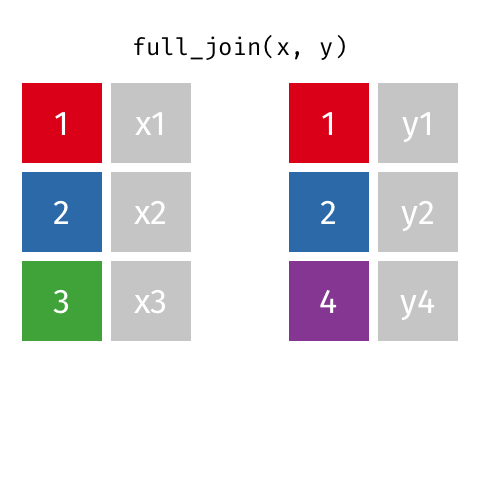
data_A.merge(data_B,how="outer")
Out[98]:
country var1 var2
0 Nigeria 4.0 low
1 England 3.0 NaN
2 Botswana 6.0 medium
3 United States NaN high
In [99]:
pd.merge(left=data_A,right=data_B,how="outer")
Out[99]:
country var1 var2
0 Nigeria 4.0 low
1 England 3.0 NaN
2 Botswana 6.0 medium
3 United States NaN high

Anti Join

In [100]:
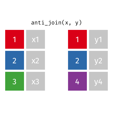
m = pd.merge(left=data_A, right=data_B, how='left', indicator=True)
m
Out[100]:
country var1 var2 _merge
0 Nigeria 4 low both
1 England 3 NaN left_only
2 Botswana 6 medium both
In [101]:
m.loc[m._merge=="left_only",:].drop(columns="_merge")
Out[101]:
country var1 var2
1 England 3 NaN

Handling disparate column names

In [102]:
D1 = pd.DataFrame(dict(cname="Russia Nigeria USA Australia".split(),
                       var1=[1,2,3,4]))
D2 = pd.DataFrame(dict(country="Belgium USA Nigeria  Botswana".split(),
                       var2=[-1,.3,2.2,1.7]))
display(D1)
D2
cname var1
0 Russia 1
1 Nigeria 2
2 USA 3
3 Australia 4
Out[102]:
country var2
0 Belgium -1.0
1 USA 0.3
2 Nigeria 2.2
3 Botswana 1.7
In [103]:
pd.merge(left = D1,
         right = D2,
         how = "outer",      # The type of join
         left_on = "cname",  # The left column naming convention 
         right_on="country") # The right column naming convention 
Out[103]:
cname var1 country var2
0 Russia 1.0 NaN NaN
1 Nigeria 2.0 Nigeria 2.2
2 USA 3.0 USA 0.3
3 Australia 4.0 NaN NaN
4 NaN NaN Belgium -1.0
5 NaN NaN Botswana 1.7

Binding Columns and Rows

row bind

In [104]:
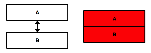
pd.concat([data_A,data_B],sort=False)
Out[104]:
country var1 var2
0 Nigeria 4.0 NaN
1 England 3.0 NaN
2 Botswana 6.0 NaN
0 Nigeria NaN low
1 United States NaN high
2 Botswana NaN medium

column bind

In [105]:
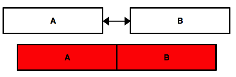
pd.concat([data_A,data_B],axis=1,sort=False)
Out[105]:
country var1 country var2
0 Nigeria 4 Nigeria low
1 England 3 United States high
2 Botswana 6 Botswana medium

Column binding with labeled indices

Essentially mimics the full join.

In [106]:
data_A2 = data_A.set_index("country")
data_B2 = data_B.set_index("country")
In [107]:
pd.concat([data_A2,data_B2],axis=1,sort=False)
Out[107]:
var1 var2
Nigeria 4.0 low
England 3.0 NaN
Botswana 6.0 medium
United States NaN high

Note that when we row bind two DataFrame objects, pandas will preserve the indices. This can result in duplicative row entries that are undesirable (not tidy).

In [108]:
pd.concat([data_A2,data_B2],axis=0,sort=False)
Out[108]:
var1 var2
country
Nigeria 4.0 NaN
England 3.0 NaN
Botswana 6.0 NaN
Nigeria NaN low
United States NaN high
Botswana NaN medium

To keep the data tidy, we can preserve which data is coming from where by generating a hierarchical index using the key argument. Put differently, we can keep track of which data is coming from where and effectively change the unit of observation from "country" to "dataset-country".

In [109]:
pd.concat([data_A2,data_B2],axis=0,sort=False,keys=["data_A2","data_B2"])
Out[109]:
var1 var2
country
data_A2 Nigeria 4.0 NaN
England 3.0 NaN
Botswana 6.0 NaN
data_B2 Nigeria NaN low
United States NaN high
Botswana NaN medium

Lastly, note that we can completely ignore the index if need be.

In [110]:
pd.concat([data_A2,data_B2],axis=0,sort=False,ignore_index=True)
Out[110]:
var1 var2
0 4.0 NaN
1 3.0 NaN
2 6.0 NaN
3 NaN low
4 NaN high
5 NaN medium