class: center, middle, inverse, title-slide # <font class = "title-panel"> PPOL561 | Accelerated Statistics for Public Policy II</font> <font size=6, face="bold"> Week 10 </font> <br> <br> <font size=100, face="bold"> Matching </font> ### <font class = "title-footer"> Prof. Eric Dunford ◆ Georgetown University ◆ McCourt School of Public Policy ◆ <a href="mailto:eric.dunford@georgetown.edu" class="email">eric.dunford@georgetown.edu</a></font> --- layout: true <div class="slide-footer"><span> PPOL561 | Accelerated Statistics for Public Policy II           Week 10 <!-- Week of the Footer Here -->              Matching <!-- Title of the lecture here --> </span></div> --- class: outline # Outline for Today ![:space 3] - **Model Dependency** ![:space 3] - **Matching** ![:space 3] - **Matching Methods** ![:space 3] - **Simulation** Example --- class: newsection ### Model Dependency --- ### Experiments ![:space 1] Valid and relatively straightforward causal inferences can be achieved via classical randomized experiments. -- ![:space 1] A good experiment requires 3 components: - **(1)** __ of units to be observed from a given population, - **(2)** __ of values of the treatment to each observed unit - **(3)** __ size ( `\(N\)` ) --- ### Experiments ![:space 1] Valid and relatively straightforward causal inferences can be achieved via classical randomized experiments. ![:space 1] A good experiment requires 3 components: - **(1)** __ by identifying a given population and guaranteeing that the probability of selection from this population is related to the potential outcomes only by random chance. - **(2)** __ even without any control variables included. - **(3)** __, i.e. imbalance. -- <br> >This is the  of causal inference --- ### Observational Research - Any data collection that  to meet the 3 experimental criteria. - Researchers analyzing observational data are instead **_forced to make assumptions_** that, if correct, help them avoid various threats to the validity of their causal inferences. -- - ****: - _Selection Bias_; - _Sufficient information on pre-treatment control variables `\(X_i\)`_; - _Pre-treatment variables are, in fact, pre-treatment_ (i.e. not influenced by the treatment); - _Independence of units_ (i.e. in time and space); - _Treatment administered to each unit is the same_ --- ### Experimental Data In experiments, **_random assignment breaks the link_** between `\(T_i\)` and `\(X_i\)` eliminating the problem of model dependence. ![:space 5] `$$E[y_i(1) | T_i = 1] = \beta_0 + \beta_1 T_i$$` `$$E[y_i(0) | T_i = 0] = \beta_0$$` ![:space 5] $$ \beta_0 + \beta_1 T_i - \beta_0$$ $$ \beta_1$$ --- ### Observational Data With observational data, we are less fortunate. We have to model the **_full functional relationship_** that connects the mean as it varies as a function of `\(T_i\)` and `\(X_i\)` over observations. ![:space 2] `$$E[y_i(1) | T_i = 1, X_i] = g(\beta_0 + \beta_1 T_i + \beta X_i)$$` `$$E[y_i(0) | T_i = 0, X_i] = g(\beta_0 + \beta X_i)$$` where - `\(g(\cdot)\)` is the assumed functional form (e.g. linear relationship) - `\(\beta_1\)` is the average treatment effect --- ### Observational Data With observational data, we are less fortunate. We have to model the **_full functional relationship_** that connects the mean as it varies as a function of `\(T_i\)` and `\(X_i\)` over observations. ![:space 5] Since `\(X_i\)` is multidimensional, this is surprisingly difficult. ![:space 5] The problem is the **_curse of dimensionality_** and the consequence in practice is **__**. --- ### Model Dependence In parametric causal inference of observational data, **_many assumptions about many parameters_** are frequently necessary. -- ![:space 3] **_Only rarely_** do we have sufficient external information to make these assumptions based on genuine knowledge. -- ![:space 3] The frequent, unavoidable consequence is **_high levels of model dependence_**. -- ![:space 3] .center[ ****. ] --- ![:space 9] <img src="week10-matching-ppol561_files/figure-html/unnamed-chunk-1-1.png" style="display: block; margin: auto;" /> --- $$ \hat{y}_i = \hat{\beta}_0 + \hat{\beta}_1 T_i + \hat{\beta}_2 x_i $$ <img src="week10-matching-ppol561_files/figure-html/unnamed-chunk-2-1.png" style="display: block; margin: auto;" /> --- $$ \hat{y}_i = \hat{\beta}_0 + \hat{\beta}_1 T_i + \hat{\beta}_2 x_i + \hat{\beta}_3 x^2_i $$ <img src="week10-matching-ppol561_files/figure-html/unnamed-chunk-3-1.png" style="display: block; margin: auto;" /> --- ### Model Dependence ![:space 2] .center[ **Imbalance<br><br>↓<br>** ] -- .center[ **** ] -- .center[ **** ] -- .center[ **__** ] --- class: newsection ### Matching --- ![:space 3] .center[ **Imbalance <br><br>↓<br><br>   __ ** ] --- ![:space 3] .center[ **~~Im~~balance   __ ** ] -- .center[ **_Central aim of statistics (and most methodologies) is to remove (or minimize) human discretion in the analytic process_** ] --- ### Matching as Nonparametric Preprocessing ![:space 3] The idea is to **adjust the data _prior_ to any parametric analysis**. -- ![:space 1] - **(1)** Eliminate or reduce the relationship between `\(T_i\)` and `\(X_i\)` -- - **(2)** Minimizes various forms of bias and inefficiency -- - **(3)** Reduces model dependencies - No longer need to model the full parametric relationship between the outcome and `\(X_i\)` - model dependence is not eliminated but will normally be greatly reduced --- ### What is Matching? ![:space 3] $$ TE_i = y_i(1) - y_i(0)$$ -- $$ TE_i = y_i(1) - \color{lightgrey}{y_i(0)}$$ -- $$ TE_i = \text{observed} - \color{lightgrey}{\text{unobserved}}$$ -- ![:space 2] We need to **_locate a suitable proxy_** for the counter-factual `\(y_i(0)\)` We can estimate `\(y_i(0)\)` by finding a suitable "match" (some `\(y_j\)` ) that can function as a control. -- We do this by **_finding observations that are "close" in the covariate space_**. $$ X_i \approx X_j $$ --- ### What is Matching? ![:space 3] `$$\widetilde {p}(X| T = 1) = \widetilde {p}(X| T = 0)$$` -- ![:space 2] The fundamental rule is to avoid **selection bias** when matching. -- - **** ("Selection on the Dependent Variable") -- - Select observations using the **** -- - Can ****, ****, or selectively **** observations from an existing sample without bias -- - If all treated units are matched, this procedure **_eliminates all dependence on the functional form_** in the parametric analysis. --- ### What is Matching? ![:space 3] `$$\widetilde {p}(X| T = 1) = \widetilde {p}(X| T = 0)$$` ![:space 3] The equation only requires that the **_distributions_ be equivalent.** -- - Matching does not require **_pairing observations_** (e.g. one-for-one exact match). More appropriate to call the method **_"pruning"_** -- - Pruning nonmatches makes **_control variables matter less_** -- - Finding matches is often most severe if `\(X_i\)` is **_high dimensional_** ("curse of dimensionality") -- .center[ > **** ] --- <img src="week10-matching-ppol561_files/figure-html/unnamed-chunk-4-1.png" style="display: block; margin: auto;" /> --- <img src="week10-matching-ppol561_files/figure-html/unnamed-chunk-5-1.png" style="display: block; margin: auto;" /> --- ### Paradoxical Advantages of Discarding Data Consider a simple linear regression with one treatment variable, `\(T_i\)` , and one covariate, `\(X_i\)`. ![:space 3] `$$var(\hat{\beta}_T) = \frac{\hat{\sigma}^2}{N(1-R^2_T) var(T_i)}$$` -- ![:space 3] If matching improves balance, then the dependence between `\(T_i\)` and `\(X_i\)` will drop - `\(R^2_T\)` will be smaller (reducing variance) -- - `\(N\)` might be smaller too (increasing variance) --- ### Paradoxical Advantages of Discarding Data ![:space 3] - Variance of the causal effect is mostly a function of the number of treated units, dropping control units (to approximate the number of treated units) -- - Even if `\(N\)` is reduced, the variance increases (even as `\(R^2_T\)` decreases), matching will still be advantageous in terms of mean squared error (unless `\(N\)` drops really low). -- - Can increase the efficiency of estimates - "More data are better" only when the estimator is based on the correct model. - When this isn't the case, estimators can have variance reductions when discarding data. --- ### The Aim of Matching - Immediate goal of matching is to **_improve balance_** -- ![:space 3] - Assessing balance is the **_main diagnostic of success_**... - ...as well as the **_number of observations_** remaining after matching ![:space 3] -- - One should **_try as many matching solutions as possible_** and choose the one with the best balance as the final preprocessed data set. - Then use the matched data set in your analysis **_using the parametric model of preference_**. --- class: newsection ### Matching Methods --- ### Matching Methods ![:space 3] There are many ways to match data. Here we'll cover a few (common) ways to do this. ![:space 3] - Exact Match - Coarsened Exact Match - Mahalanobis Distance Matching - Propensity Score Matching (Most Common) ![:space 3] Consults the Ho. et al. JSS article (suggested reading) for an overview of all matching implementations using `MatchIt`. --- .center[ ### Exact Match ] <img src="week10-matching-ppol561_files/figure-html/unnamed-chunk-6-1.png" style="display: block; margin: auto;" /> --- .center[ ### Exact Match ] <img src="week10-matching-ppol561_files/figure-html/unnamed-chunk-7-1.png" style="display: block; margin: auto;" /> --- ### Coarsened Exact Match ![:space 5 ] - **_Temporarily "coursen"_** (bin) `\(X\)` as much as possible (or willing) -- - **_Apply exact matching_** to coarsened `\(X, C(X)\)` - Sort observations into strata, each with unique values of `\(C(X)\)` - Prune any stratum with 0 treated or 0 control units -- - **_Pass on original (uncoarsened) units_** except those pruned -- - When estimating model, **weight** each treated to each control. -- - The approach approximates Fully Blocked Experiment. Very Powerful! --- .center[ ### Coarsened Exact Match ] <img src="week10-matching-ppol561_files/figure-html/unnamed-chunk-8-1.png" style="display: block; margin: auto;" /> --- .center[ ### Coarsened Exact Match ] <img src="week10-matching-ppol561_files/figure-html/unnamed-chunk-9-1.png" style="display: block; margin: auto;" /> ![:space 25] ``` ## ## Using 'treat'='1' as baseline group ``` --- .center[ ### Coarsened Exact Match ] <img src="week10-matching-ppol561_files/figure-html/unnamed-chunk-11-1.png" style="display: block; margin: auto;" /> --- ### Mahalanobis Distance Matching ![:space 2] **Mahalanobis distance** is a measure of the distance between a point and a distribution. It is a **_multi-dimensional generalization_** of the idea of measuring how many standard deviations away a point is from the mean of a distribution. $$ D(X_i, X_j) = \sqrt{(X_i - X_j)S^{-1}(X_i - X_j)} $$ - More generally, we use Euclidean (or other distance metrics). - The idea is to **_match each treated unit to the "closest" control unit_**. - **_Prune matches_** if Distance > caliper (threshold cutoff). --- .center[ ### Mahalanobis Distance Matching ]  --- .center[ ### Mahalanobis Distance Matching ]  --- .center[ ### Mahalanobis Distance Matching ]  --- .center[ ### Mahalanobis Distance Matching ]  --- .center[ ### Mahalanobis Distance Matching ]  --- ### Propensity Score Matching ![:space 2] Reduce the `\(p\)` variables of `\(X\)` to a **_scalar_** $$ \pi_i = pr(T_i = 1| X) = \frac{1}{1+e^{-X_i\beta}} $$ -- - The idea is to **_model the randomization process_** (the probability of being randomly assigned to the treatment and/or control) -- - Match each treated unit to the nearest control unit $$ D(X_i,X_j) = |\pi_i - \pi_j| $$ -- - Prune matches if Distance > caliper -- - By far the most commonly used matching method --- .center[ ### Propensity Score Matching ]  --- .center[ ### Propensity Score Matching ]  --- .center[ ### Propensity Score Matching ]  --- .center[ ### Propensity Score Matching ] 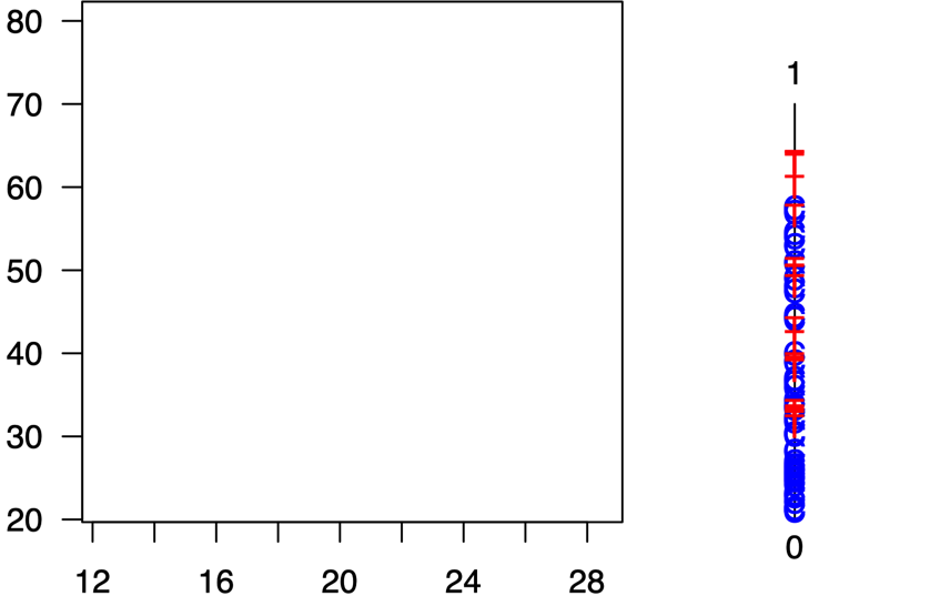 --- .center[ ### Propensity Score Matching ] 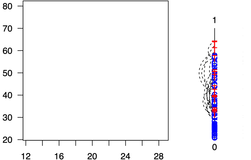 --- .center[ ### Propensity Score Matching ] 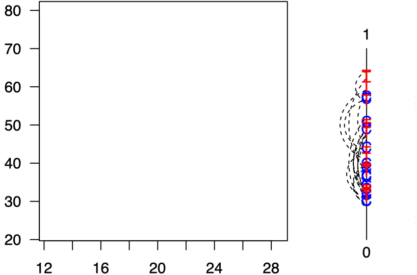 --- .center[ ### Propensity Score Matching ] 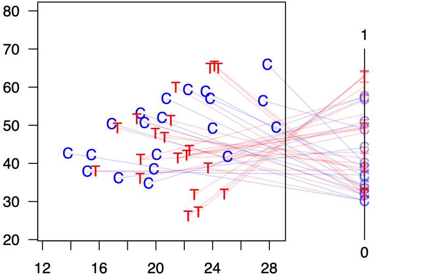 --- .center[ ### Propensity Score Matching ]  --- ### The Propensity Score Matching Paradox - Recall **_randomization can result in imbalance_** (even under the best circumstances) -- - Propensity Score Matching **_approximates complete randomization_**... meaning it can _increase_ imbalance in data at times. -- - Problem grows as the **_dimensionality_** in `\(X\)` grows. -- - Recent push to away from propensity scores - See "Why Propensity Scores Should Not Be Used for Matching" (suggested reading) - Suggest using methods that approximate a fully blocked experiment, like coursened exact matching --- ### The Matching Frontier .center[ **Bias-Variance `\(\approx\)` Imbalance-N** ] - There are many matching methods one can try. -- ![:space 1] - One should try all and see which yields the best matching sample. Quickly making this exercise an optimization problem! -- ![:space 1] - Need to ensure optimality: i.e. we want to live in a world where no cherry picking is possible. -- ![:space 1] - "Matching Frontier" Method scans all possible matching combinations and presents the "frontier" with the most optimal matches given pruning. - See "The Balance-Sample Size Frontier in Matching Methods for Causal Inference" ( King et al. 2017) --- class: newsection ### Simulation Example --- ### Aim of the Simulation - See how well these methods perform on "known" data - Explore implementing the different matching methods --- ![:space 3] ```r set.seed(123) # Seed for replication N = 1000 # Sample Size # Random explanatory variables x1 <- rnorm(N) x2 <- rnorm(N) # Probability of being in the treatment group is a # function of existing covariates z = -1 + x1 + x2 # Linear combination w/r/t pr(T=1) pr_tr <- pnorm(z) # Probability of being treated tr <- rbinom(N,1,pr_tr) # 1, 0 -> treated or not # Treatment is correlated with covariates # Outcome (TREATMENT EFFECT == 1) y = tr + x1*x2 + x1^2 + x1^3 + rnorm(N) # Gather as a data frame D = tibble(y,x1,x2,tr) ``` --- ```r pairs(D,col="steelblue") ``` <img src="week10-matching-ppol561_files/figure-html/unnamed-chunk-13-1.png" style="display: block; margin: auto;" /> --- ```r td = function(...) broom::tidy(...) %>% mutate_if(is.numeric,function(x) round(x,2)) m1 <- lm(y ~ tr,data=D) td(m1) ``` ``` ## # A tibble: 2 x 5 ## term estimate std.error statistic p.value ## <chr> <dbl> <dbl> <dbl> <dbl> ## 1 (Intercept) 0.18 0.14 1.22 0.22 ## 2 tr 4.78 0.28 17.1 0 ``` -- ```r m2 <- lm(y ~ tr + x1 + x2,data=D) td(m2) ``` ``` ## # A tibble: 4 x 5 ## term estimate std.error statistic p.value ## <chr> <dbl> <dbl> <dbl> <dbl> ## 1 (Intercept) 0.85 0.12 7.16 0 ## 2 tr 2.08 0.28 7.47 0 ## 3 x1 2.77 0.11 25.3 0 ## 4 x2 -0.07 0.11 -0.66 0.51 ``` --- ### Treatment effect can be recovered... ...If we know the functional form of the "true model" (i.e. the underlying data generating process) -- ```r m3 <- lm(y ~ tr + x1*x2 + I(x1^2) + I(x1^3),data=D) td(m3) ``` ``` ## # A tibble: 7 x 5 ## term estimate std.error statistic p.value ## <chr> <dbl> <dbl> <dbl> <dbl> ## 1 (Intercept) 0.03 0.04 0.76 0.45 ## 2 tr 0.92 0.1 9.6 0 ## 3 x1 -0.07 0.06 -1.12 0.26 ## 4 x2 0.06 0.04 1.65 0.1 ## 5 I(x1^2) 0.99 0.02 40.6 0 ## 6 I(x1^3) 1.02 0.02 64.6 0 ## 7 x1:x2 0.97 0.03 29.2 0 ``` -- We rarely if ever know this... --- ```r # Propensity Score Matching m_out = matchit(tr ~ x1 + x2, method="nearest", distance = "logit", discard = "both", data=D) m_out$nn ``` ``` ## Control Treated ## All 734 266 ## Matched 220 220 ## Unmatched 407 0 ## Discarded 107 46 ``` -- ```r summary(m_out) ``` ``` ## ## Call: ## matchit(formula = tr ~ x1 + x2, data = D, method = "nearest", ## distance = "logit", discard = "both") ## ## Summary of balance for all data: ## Means Treated Means Control SD Control Mean Diff eQQ Med eQQ Mean ## distance 0.6234 0.1365 0.1888 0.4869 0.5456 0.4869 ## x1 0.7528 -0.2508 0.8874 1.0036 0.9942 1.0064 ## x2 0.8389 -0.2462 0.9110 1.0850 1.0576 1.0877 ## eQQ Max ## distance 0.7204 ## x1 1.3044 ## x2 1.5018 ## ## ## Summary of balance for matched data: ## Means Treated Means Control SD Control Mean Diff eQQ Med eQQ Mean ## distance 0.5513 0.3610 0.2059 0.1903 0.2044 0.1903 ## x1 0.5832 0.3178 0.7452 0.2654 0.2527 0.2675 ## x2 0.6845 0.4568 0.7129 0.2277 0.2296 0.2299 ## eQQ Max ## distance 0.3521 ## x1 0.5758 ## x2 0.5161 ## ## Percent Balance Improvement: ## Mean Diff. eQQ Med eQQ Mean eQQ Max ## distance 60.9273 62.5342 60.9141 51.1305 ## x1 73.5535 74.5810 73.4191 55.8526 ## x2 79.0135 78.2879 78.8659 65.6359 ## ## Sample sizes: ## Control Treated ## All 734 266 ## Matched 220 220 ## Unmatched 407 0 ## Discarded 107 46 ``` --- ```r plot(m_out,type="hist") ``` <img src="week10-matching-ppol561_files/figure-html/unnamed-chunk-19-1.png" style="display: block; margin: auto;" /> --- ![:space 15] ```r D_m = match.data(m_out) head(D_m) ``` ``` ## y x1 x2 tr distance weights ## 3 6.4840246 1.5587083 -0.01798024 1 0.6497653 1 ## 7 1.4010378 0.4609162 0.24972574 1 0.3035990 1 ## 8 -1.4618409 -1.2650612 2.41620737 1 0.5739433 1 ## 14 -0.4309013 0.1106827 0.46903196 0 0.2628795 1 ## 16 8.7310388 1.7869131 0.18705115 0 0.8065223 1 ## 17 1.7727020 0.4978505 0.22754273 1 0.3084882 1 ``` ```r dim(D_m) ``` ``` ## [1] 440 6 ``` --- ```r D_m %>% select(x1,x2,tr) %>% gather(var,val,-tr) %>% ggplot(aes(val,fill=factor(tr))) + geom_histogram(alpha=.7) + facet_wrap(~var,ncol = 2) ``` <img src="week10-matching-ppol561_files/figure-html/unnamed-chunk-22-1.png" style="display: block; margin: auto;" /> --- ![:space 15] ```r D_m %>% group_by(tr) %>% summarize(x1 = mean(x1), x2 = mean(x2)) ``` ``` ## # A tibble: 2 x 3 ## tr x1 x2 ## <int> <dbl> <dbl> ## 1 0 0.318 0.457 ## 2 1 0.583 0.685 ``` --- ![:space 5] ```r td(lm(y ~ tr , data=D_m)) ``` ``` ## # A tibble: 2 x 5 ## term estimate std.error statistic p.value ## <chr> <dbl> <dbl> <dbl> <dbl> ## 1 (Intercept) 1.15 0.26 4.42 0 ## 2 tr 2.31 0.37 6.27 0 ``` ```r td(lm(y ~ tr + x1 + x2, data=D_m)) ``` ``` ## # A tibble: 4 x 5 ## term estimate std.error statistic p.value ## <chr> <dbl> <dbl> <dbl> <dbl> ## 1 (Intercept) -0.290 0.2 -1.43 0.15 ## 2 tr 1.16 0.24 4.82 0 ## 3 x1 4.06 0.18 23.1 0 ## 4 x2 0.33 0.19 1.78 0.08 ``` --- ![:space 15] ```r # Mahalanobis Distance Matching m_out2 = matchit(tr ~ x1 + x2, data=D, method="nearest", distance="mahalanobis", discard = "both") # Generate a matched data frame D_m2 = match.data(m_out2) m_out2$nn ``` ``` ## Control Treated ## All 734 266 ## Matched 266 266 ## Unmatched 468 0 ## Discarded 0 0 ``` --- ```r D_m2 %>% select(x1,x2,tr) %>% gather(var,val,-tr) %>% ggplot(aes(val,fill=factor(tr))) + geom_histogram(alpha=.7) + facet_wrap(~var,ncol = 2) ``` <img src="week10-matching-ppol561_files/figure-html/unnamed-chunk-26-1.png" style="display: block; margin: auto;" /> --- ![:space 15] ```r D_m2 %>% group_by(tr) %>% summarize(x1 = mean(x1), x2 = mean(x2)) ``` ``` ## # A tibble: 2 x 3 ## tr x1 x2 ## <int> <dbl> <dbl> ## 1 0 0.297 0.373 ## 2 1 0.753 0.839 ``` --- ![:space 5] ```r td(lm(y ~ tr , data=D_m2)) ``` ``` ## # A tibble: 2 x 5 ## term estimate std.error statistic p.value ## <chr> <dbl> <dbl> <dbl> <dbl> ## 1 (Intercept) 1.03 0.31 3.35 0 ## 2 tr 3.93 0.43 9.06 0 ``` ```r td(lm(y ~ tr + x1 + x2, data=D_m2)) ``` ``` ## # A tibble: 4 x 5 ## term estimate std.error statistic p.value ## <chr> <dbl> <dbl> <dbl> <dbl> ## 1 (Intercept) -0.92 0.22 -4.25 0 ## 2 tr 1.05 0.3 3.47 0 ## 3 x1 5.21 0.18 28.6 0 ## 4 x2 1.08 0.19 5.63 0 ``` --- ![:space 15] ```r # Course Exact Matching m_out3 = matchit(tr ~ x1 + x2, method="cem", discard = "both", data=D) ``` ``` ## ## Using 'treat'='1' as baseline group ``` ```r # Generate a matched data frame D_m3 = match.data(m_out3) m_out3$nn ``` ``` ## Control Treated ## All 734 266 ## Matched 485 235 ## Unmatched 143 10 ## Discarded 106 21 ``` --- ```r D_m3 %>% select(x1,x2,tr) %>% gather(var,val,-tr) %>% ggplot(aes(val,fill=factor(tr))) + geom_histogram(alpha=.7) + facet_wrap(~var,ncol = 2) ``` <img src="week10-matching-ppol561_files/figure-html/unnamed-chunk-30-1.png" style="display: block; margin: auto;" /> --- ![:space 15] ```r D_m3 %>% group_by(tr) %>% summarize(x1 = mean(x1*weights), x2 = mean(x2*weights)) ``` ``` ## # A tibble: 2 x 3 ## tr x1 x2 ## <int> <dbl> <dbl> ## 1 0 0.647 0.628 ## 2 1 0.692 0.725 ``` --- ![:space 5] ```r td(lm(y ~ tr , weights = D_m3$weights, data=D_m3)) ``` ``` ## # A tibble: 2 x 5 ## term estimate std.error statistic p.value ## <chr> <dbl> <dbl> <dbl> <dbl> ## 1 (Intercept) 2.77 0.21 13.0 0 ## 2 tr 1.31 0.37 3.5 0 ``` ```r td(lm(y ~ tr + x1 + x2,weights = D_m3$weights, data=D_m3)) ``` ``` ## # A tibble: 4 x 5 ## term estimate std.error statistic p.value ## <chr> <dbl> <dbl> <dbl> <dbl> ## 1 (Intercept) -0.39 0.18 -2.13 0.03 ## 2 tr 1.08 0.2 5.31 0 ## 3 x1 4.8 0.12 39.5 0 ## 4 x2 0.09 0.15 0.61 0.54 ``` --- ### Keep in mind - Matching is a preprocessing step useful to reduce model dependency by generating a balanced dataset. - Not all matching methods are created equal. - Need to explore different methods to see which one provides the best balance. - New methods emerging that aid in locating the optimal match. - When balancing, one must have all the covariates that related to the treatment assignment and the outcome. - If you lack complete data, this can be a source of bias (i.e. you're not balancing on the dimensions that matter) - Balancing becomes more difficult as the dimensionality of `\(X\)` increases.